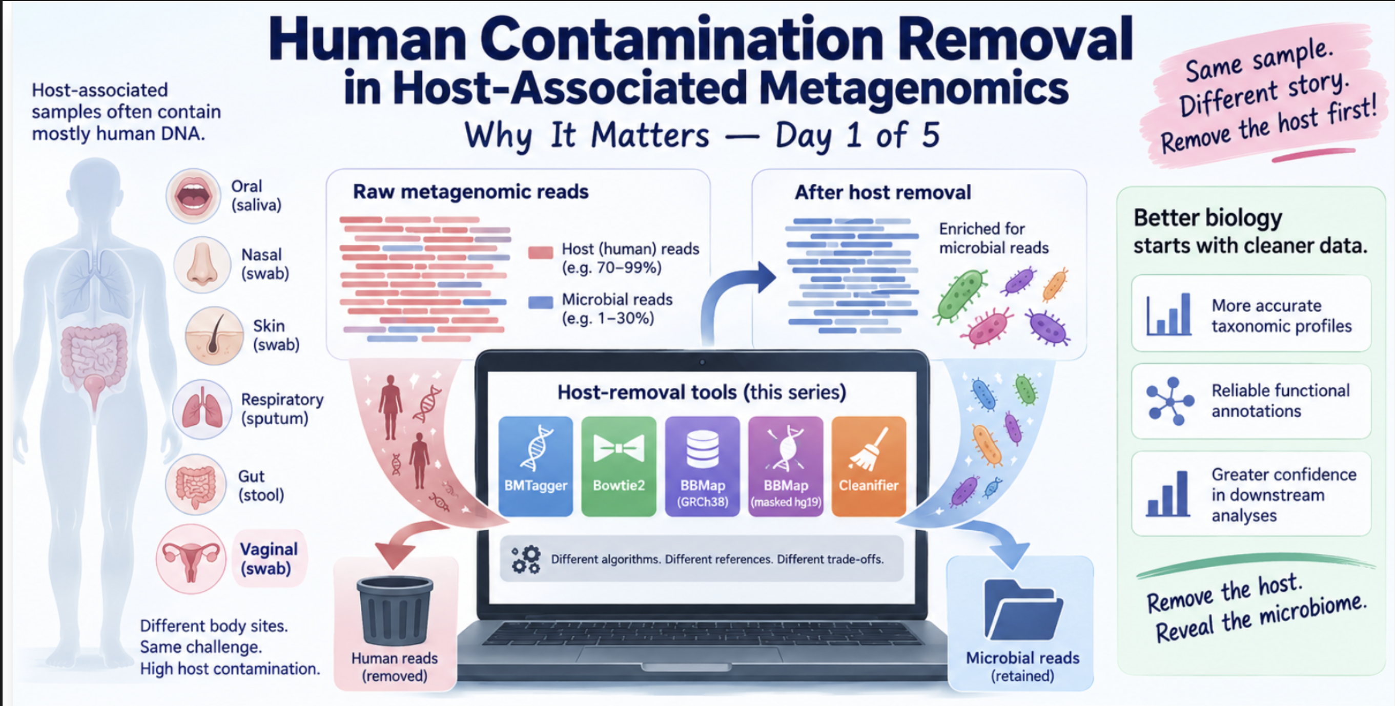
Human Contamination Removal in Host-Associated Metagenomics: Why It Matters — Day 1 of 5
🧬 Day 1 of 5 — Benchmarking Host-Read Removal for High-Host-Content Metagenomes
Shotgun metagenomics gives us access to microbial genomes, functional pathways, strain-level variation, and the full metabolic potential of a community — things that amplicon sequencing cannot reach. But in host-associated samples, one practical problem appears before almost any of that biology can begin: a substantial fraction of your sequencing reads may come from the host rather than the microbiome.
This is not a minor calibration issue. In some vaginal swab datasets, host-derived reads can account for the majority of the library. Process them without removing host reads first, and every downstream step — taxonomic profiling, differential abundance, functional annotation — is working with a contaminated input. Worse, the contamination is not random noise; it is a structured signal from a specific organism (you), which can create systematic artifacts in community profiles.
The standard solution is to run a host-removal step before anything else. Map your reads to the human reference genome, discard the matches, keep the rest. Simple in principle. But the question of which tool to use, with which reference, evaluated against which criteria — that is less simple than it sounds, and the choices have real consequences for the biology you ultimately report.
This post opens a five-day benchmarking series. Over the week I will run five host-removal strategies on five vaginal metagenomes, measure what each tool removes, what it retains, how fast it runs, how much memory it needs, and — most importantly — whether the reads it discards are actually human or microbial. Today is the framing: why this benchmark exists, what it measures, and what a rigorous host-removal evaluation actually needs to look at.
The two ways a host-removal tool can fail
Every host-removal method can make two types of error, and they are not symmetric in their consequences.
Error type 1: Retaining human reads. The tool misses reads that are genuinely from the host. These contaminate your microbial profile — false taxa, inflated diversity, spurious functional signals. This is the error most people think about.
Error type 2: Removing microbial reads. The tool discards reads that are genuinely from the microbiome because they share sequence similarity with the human reference. This is the error that is easy to overlook — especially when you are looking at a summary table where the fraction of incorrectly removed reads appears tiny.
The second error is the more insidious one, because its consequences are invisible in the host-removal output itself. You only see it later, downstream, when a biologically important taxon appears underrepresented or absent — and you have no easy way to know whether that is a real biological signal or an artifact of your decontamination step.
Why vaginal metagenomics is a particularly challenging case
Vaginal microbial communities are ecologically unusual. Unlike gut communities, which are highly diverse and numerically dominated by many taxa, vaginal communities can be dominated by a small number of biologically critical organisms. Depending on the individual and community state type, a sample might be overwhelmingly composed of just one or two species:
- Lactobacillus iners — the most prevalent vaginal Lactobacillus, associated with community instability
- Lactobacillus crispatus — associated with community stability and health
- Gardnerella spp. — key players in bacterial vaginosis
- Sneathia vaginalis, Fannyhessea vaginae, Aerococcus christensenii — associated with BV and adverse reproductive outcomes
- Metamycoplasma hominis — a common BV-associated organism with an unusual genome
This low-diversity, high-dominance structure means that if a host-removal tool systematically discards reads from even one of these taxa — because those reads share a short region of sequence similarity with the human genome — the biological impact is disproportionately large. The overall false-positive removal rate in your summary statistics might be 0.1%. The impact on your L. iners abundance estimate might be 15%.
The question is therefore not simply “which tool removes the most reads?” A more precise question is:
Which method provides the best balance between human-read removal sensitivity, microbial-read specificity, runtime, memory use, and workflow reproducibility — at the sample-level host content typical of vaginal specimens?
The benchmark design
Five paired-end vaginal metagenomes were selected to span a broad range of host contamination levels. All sample identifiers are anonymized for this public technical series.
| Sample | Input read pairs | Host content category |
|---|---|---|
| Sample 1 | 41,644,670 | Very high |
| Sample 2 | 43,344,280 | Very high |
| Sample 3 | 41,089,173 | Moderate |
| Sample 4 | 31,349,380 | Low |
| Sample 5 | 37,060,999 | High |
| Total | 194,488,502 | — |
The range matters. A tool that performs well on a low-host sample might struggle on a very high-host sample, or vice versa. Evaluating across this range gives a more honest picture of how each method scales with the biological reality of the input.
Standardizing the input: fastp first
Before any host-removal tool saw the data, all samples were processed with fastp — quality trimming, adapter removal, quality filtering. Every host-removal method then received exactly the same quality-controlled reads.
This step is non-negotiable for a fair comparison. If method A receives raw reads and method B receives trimmed reads, you are measuring two different things simultaneously and cannot attribute differences in outcome to the host-removal algorithm. Standardizing input is the first rule of tool benchmarking.
fastp \
  --in1 sample_R1.fastq.gz \
  --in2 sample_R2.fastq.gz \
  --out1 sample_fastp_R1.fastq.gz \
  --out2 sample_fastp_R2.fastq.gz \
  --json sample_fastp.json \
  --html sample_fastp.html \
  --thread 8 \
  --detect_adapter_for_pe \
  --qualified_quality_phred 20 \
  --length_required 50
The five methods being compared
| Method | Strategy | Why it is included |
|---|---|---|
| BMTagger | Legacy k-mer screening + alignment | Historical baseline; still used in some lab workflows |
| Bowtie2 | FM-index alignment to GRCh38 | Widely used conventional approach |
| BBMap + GRCh38 | k-mer-seeded hybrid mapping | Flexible, high-sensitivity mapper against standard reference |
| BBMap + masked hg19 | Hybrid mapping to repeat-masked reference | Tests whether reference masking changes removal rates |
| Cleanifier | Modern probabilistic filtering, pangenome-aware | Very fast; designed for clinical and high-host-content samples |
One thing that became clear immediately while planning this benchmark: the reference genome can matter almost as much as the aligner. BBMap run against GRCh38 is not the same as BBMap run against a repeat-masked hg19 reference. The algorithm is identical; the database is different. Both comparisons belong in a rigorous evaluation, which is why BBMap appears twice.
This means the benchmark is measuring two things simultaneously:
- Algorithm effects — does the underlying alignment or classification strategy matter?
- Reference effects — does the choice of human reference change what gets removed?
What the benchmark measures
A single “percentage of reads removed” number is not enough. For each tool on each sample, I tracked:
| Metric | Why it matters |
|---|---|
| % read pairs classified as human | Primary removal rate |
| Retained non-human read pairs | What goes into downstream analysis |
| Wall-clock runtime | Practical compute cost |
| Peak RAM (maximum resident set size) | Determines whether tool runs on a laptop vs HPC |
| CPU usage | Efficiency of parallelization |
| Discordant pairs between methods | Reads that one tool removes but another retains — the scientifically interesting subset |
| Evidence of microbial false-positive removal | Whether any known vaginal taxa are being incorrectly discarded |
The last two metrics require extra work beyond running the tool — they require cross-comparing outputs and mapping retained/discarded reads back to taxonomic assignments. But they are the metrics that actually answer the biological question.
Measuring compute cost with /usr/bin/time -v
Every tool run was wrapped with:
/usr/bin/time -v tool_command \
  2> sample_tool_timing.txt
The -v flag (verbose mode) reports:
Elapsed (wall clock) time:    0:04:23.15
Maximum resident set size:    12,847,316 KB
User time (seconds):          187.34
System time (seconds):        6.21
Percent of CPU this job got:  73%
This is more informative than timing alone — it tells you whether the tool is memory-bound (relevant for deciding whether it can run on a standard server or requires HPC), and whether it parallelizes efficiently (relevant for estimating how long it will take at scale).
HPC infrastructure: SLURM array jobs
Benchmarking full metagenomes on a laptop is impractical. The full workflow ran on an HPC cluster organized as a SLURM array:
5 samples × 5 tool configurations = 25 benchmark jobs
Each job received the same fastp-preprocessed inputs, wrote tool-specific outputs to a structured directory, and generated three additional files per run: a timing file, a command record, and a status file.
#!/bin/bash
#SBATCH --job-name=host_removal_benchmark
#SBATCH --array=1-25
#SBATCH --cpus-per-task=16
#SBATCH --mem=64G
#SBATCH --time=12:00:00
#SBATCH --output=logs/benchmark_%A_%a.out
#SBATCH --error=logs/benchmark_%A_%a.err

# Each array task reads its sample and tool assignment from a lookup table
SAMPLE=$(sed -n "${SLURM_ARRAY_TASK_ID}p" benchmark_jobs.txt | awk '{print $1}')
TOOL=$(sed -n "${SLURM_ARRAY_TASK_ID}p" benchmark_jobs.txt | awk '{print $2}')

# Tool-specific commands are dispatched from here
bash run_${TOOL}.sh ${SAMPLE}
The benchmark_jobs.txt file is a 25-line table mapping array task IDs to sample-tool combinations. This design makes the benchmark fully auditable: every job’s exact command, input, and output is recorded, and any individual job can be rerun in isolation if needed.
The full workflow
Raw paired-end FASTQ
        ↓
fastp preprocessing (same for all methods)
        ↓
Standardized quality-controlled input
        ↓
┌──────────────────────────────────┐
│  5 host-removal tools in parallel │
│  BMTagger                         │
│  Bowtie2 → GRCh38                │
│  BBMap → GRCh38                  │
│  BBMap → masked hg19             │
│  Cleanifier                       │
└──────────────┬───────────────────┘
               ↓
   Human reads (discarded) + Retained reads
               ↓
   Runtime / RAM / removal rate per tool
               ↓
   Read-level discordance analysis
   (which reads does only one tool remove?)
               ↓
   Microbial specificity validation
   (are any vaginal taxa being falsely removed?)
               ↓
   Final comparison table
The last two steps — discordance analysis and microbial specificity validation — are the ones that distinguish a benchmark from simply running five tools and comparing numbers. Two methods can remove nearly identical percentages of reads while disagreeing substantially on which specific reads those are. If the disagreement is concentrated in reads from Gardnerella or L. iners, the two methods are not equivalent even if their removal rates look the same.
What comes next
Over the next four days:
Day 2 — BMTagger and Bowtie2: installation, reference preparation, paired-end commands, outputs, and why BMTagger remains a useful baseline despite being much slower than modern alternatives.
Day 3 — BBMap with GRCh38 and masked hg19: how to run BBMap for host removal, what the reference masking actually changes, and first results from the high-host samples.
Day 4 — Cleanifier: the newest method in the benchmark, designed specifically for high-host-content clinical metagenomes, with a pangenome-aware approach that differs substantially from the alignment-based tools.
Day 5 — Full comparison: all five methods side by side. Removal rates, runtime, RAM, discordant read analysis, and which tool performs best across the range of host content represented in these samples.
The central principle of this benchmark
The metric I am optimizing for is not maximum human-read removal. A tool that removes 99.9% of human reads while also removing 5% of Lactobacillus reads is not a better tool — it is a differently failing tool, in a way that is harder to detect and more damaging to biological interpretation.
The metric that actually matters is closer to:
High host-removal sensitivity
      +
High microbial-read specificity
      +
Reasonable compute cost
      +
Reproducible, auditable workflow
Whether any single tool achieves all four is what this benchmark will determine.
Sample identifiers have been anonymized for this public technical series. The benchmark is presented to illustrate workflow design and method comparison. Day 2 publishes soon.