Speed, Sensitivity, and Microbial Specificity: The Final Host-Removal Benchmark — Day 5 of 5
🧬 Day 5 of 5 — Benchmarking Host-Read Removal for High-Host-Content Metagenomes
This series started with a deceptively simple question: which tool should you use to remove human reads from a host-associated metagenome? Over four days, that question expanded considerably. The benchmark moved from timing comparisons and removal percentages to read-level concordance and the practical question of whether differences in filtering change downstream microbiome profiles. Today I bring all of that together.
The central lesson is one worth stating upfront: host-removal benchmarking should not be reduced to a single percentage column. The percentage of reads removed is necessary information — but it is not sufficient. A tool that removes more reads is not automatically better. A tool that runs faster is not automatically acceptable. The question is whether differences in filtering affect the microbial signal that downstream analyses are intended to measure.
The benchmark dataset
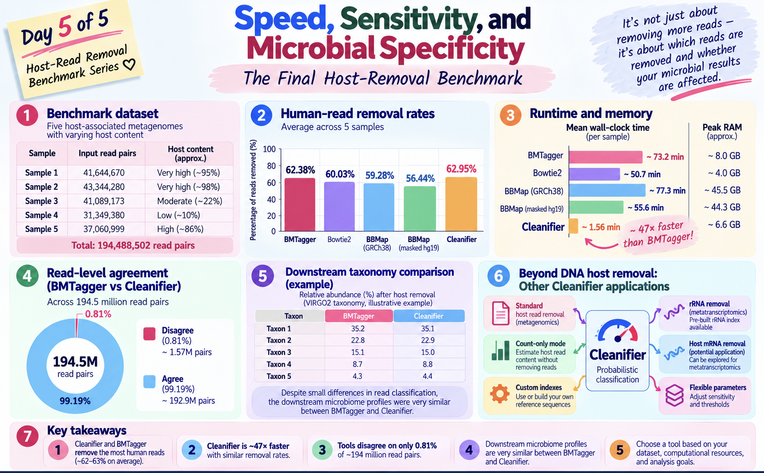
Five anonymized paired-end metagenomes processed after standardized fastp preprocessing. Total input across all samples:
194,488,502 read pairs
Host content varied substantially:
| Sample | Input read pairs | Host content |
|---|---|---|
| Sample 1 | 41,644,670 | Very high (~95%) |
| Sample 2 | 43,344,280 | Very high (~98%) |
| Sample 3 | 41,089,173 | Moderate (~22%) |
| Sample 4 | 31,349,380 | Low (~10%) |
| Sample 5 | 37,060,999 | High (~86%) |
This range was deliberate. A host-removal method needs to perform sensibly in both microbe-rich and host-dominated samples. A tool that looks excellent on a low-host sample may behave differently when 95% of the library is human.
Human-read removal rates
| Sample | BMTagger | Bowtie2 | BBMap GRCh38 | BBMap masked hg19 | Cleanifier |
|---|---|---|---|---|---|
| Sample 1 | 94.88% | 89.76% | 89.85% | 85.57% | 95.73% |
| Sample 2 | 97.91% | 94.82% | 93.26% | 88.44% | 98.88% |
| Sample 3 | 22.51% | 21.72% | 21.25% | 20.19% | 22.72% |
| Sample 4 | 10.52% | 10.14% | 9.83% | 9.30% | 10.61% |
| Sample 5 | 86.07% | 83.71% | 82.19% | 78.71% | 86.83% |
| Mean | 62.38% | 60.03% | 59.28% | 56.44% | 62.95% |
A consistent ranking emerged across all five samples:
Cleanifier ≈ BMTagger
      >
Bowtie2 ≈ BBMap GRCh38
      >
BBMap masked hg19
BBMap with the masked hg19 reference consistently removed fewer reads than BBMap with GRCh38.p12. This comparison illustrates the importance of documenting the exact reference: the two runs differed in both genome assembly and masking, so the observed difference cannot be attributed to masking alone. That was the central methodological lesson of Day 3.
But more removal is not automatically better. The table above does not tell you whether the reads each tool removes are genuinely human. That question required a different kind of analysis.
Computational performance
| Tool | Mean wall-clock runtime | Approximate peak RAM |
|---|---|---|
| BMTagger | ~73.2 min | ~8.0 GB |
| Bowtie2 | ~50.7 min | ~4.0 GB |
| BBMap GRCh38 | ~77.3 min | ~45.5 GB |
| BBMap masked hg19 | ~55.6 min | ~44.3 GB |
| Cleanifier | ~1.56 min | ~6.6 GB |
Cleanifier was approximately 47× faster than BMTagger while producing nearly identical overall removal rates. For larger cohorts, this runtime difference can substantially reduce aggregate compute time, although total wall-clock completion depends on scheduling, parallelism, and I/O.
BBMap’s RAM requirement (~45 GB) stands out as a practical constraint. On a shared HPC cluster, scheduling 45 GB per job limits how many samples run simultaneously and requires careful resource planning. Cleanifier’s ~6.6 GB footprint is comparatively easy to schedule on typical HPC nodes.
Read-level discordance analysis
Removal percentages describe aggregate behavior. They do not reveal what happens at the level of individual reads. To go deeper, I reconstructed read-pair-level classifications for BMTagger and Cleanifier — the two tools that removed the most reads — across all 194.5 million pairs.
Every read pair was placed into one of four categories:
| BMTagger | Cleanifier | Category |
|---|---|---|
| Remove | Remove | Both remove — concordant removal |
| Remove | Keep | BMTagger-only |
| Keep | Remove | Cleanifier-only |
| Keep | Keep | Neither removes — concordant retention |
The result:
| Category | Read pairs | % of total |
|---|---|---|
| Both remove | 126,193,291 | 64.88% |
| BMTagger-only | 204,189 | 0.10% |
| Cleanifier-only | 1,373,154 | 0.71% |
| Neither removes | 66,717,868 | 34.31% |
| Total discordant | 1,577,343 | 0.81% |
The two methods agree on 99.19% of all read pairs. That level of concordance is reassuring — the two tools are largely making the same calls. But the disagreement is sharply asymmetric: ~87% of all discordant pairs are Cleanifier-only removals — reads that Cleanifier removes but BMTagger retains. The asymmetry is worth documenting, but disagreement alone does not establish which classification is correct or whether a downstream taxonomic result changes.
Do different filtering decisions change downstream taxonomy?
The discordance analysis identifies where BMTagger and Cleanifier make different decisions. It does not, by itself, tell us whether those differences alter the community profile that a researcher would report. That is why an additional downstream comparison is valuable.
In this benchmark, the retained reads from BMTagger and Cleanifier were taken forward for taxonomic profiling. The downstream taxonomic profiles examined did not show noticeable differences between the two workflows. This observation is important because a small read-level disagreement need not produce a meaningful change in the taxa represented in the final abundance table. It should not, however, be interpreted as proof that every read was classified correctly or that all possible downstream analyses will agree.
A simple illustration using five fictional taxa
The table below is a toy example for explanation only. These are invented taxa labels and invented relative abundances, not measurements from the benchmark or an export of the taxonomy results. It shows what near-identical downstream profiles can look like even when the upstream host-removal tools do not classify every read pair identically.
| Illustrative taxon | BMTagger workflow | Cleanifier workflow |
|---|---|---|
| Taxon 1 | 40.0% | 40.1% |
| Taxon 2 | 30.0% | 29.9% |
| Taxon 3 | 15.0% | 15.0% |
| Taxon 4 | 10.0% | 10.0% |
| Taxon 5 | 5.0% | 5.0% |
| Total | 100.0% | 100.0% |
Illustrative values only; do not cite this table as empirical benchmark data.
The useful comparison is not merely the number of reads retained. It is whether the major taxa, their relative abundances, and the biological interpretation remain stable after the filtering step. In the profiles examined here, the downstream results were similar despite differences in read-level decisions.
For a formal publication, this comparison could be expanded with paired taxon-abundance plots, rank correlations, compositional distances, and sample-level concordance. Those additional quantitative results are not presented here; the observation above is deliberately limited to the downstream profiles that were examined.
Beyond host-read removal: what else can Cleanifier do?
The five-sample benchmark above evaluated human DNA read filtering. While preparing the final comparison, I also looked more closely at what Cleanifier can do outside that specific use case. Its underlying idea is general: compare sequencing reads with a reference index built from sequences that we want to identify or exclude. The biological interpretation depends entirely on the index being used.
Cleanifier uses spaced-seed (gapped k-mer) matching rather than conventional base-by-base alignment. Its published implementation supports paired-end and single-end FASTQ, compressed reads, a fast sampling mode, a more sensitive mode, and custom indexes. These are documented software capabilities, not additional experiments performed in this benchmark.
1. Count likely host reads before deciding to remove them
Not every analysis needs to begin by immediately writing a new host-depleted FASTQ. Sometimes the first question is simply: How much of this sequencing library appears to be host-derived?
Cleanifier includes a --count option that performs classification without writing filtered read files. This can be useful for an initial survey of a sequencing batch, for comparing the host-read burden across samples, or for prioritizing samples that might need deeper sequencing. The exact statistics printed by a particular release should be checked with its --help output and captured in the run log.
# Example: classify/count against a human index, without writing filtered FASTQ
cleanifier filter \
  --index /path/to/human_index \
  --fastq sample_R1.fastq.gz \
  --pairs sample_R2.fastq.gz \
  --prefix sample_host_screen \
  --count 2>&1 | tee sample_host_screen.log
This produces an index-based estimate of the host-associated fraction, not an independent ground-truth measurement of host DNA. A count-only screening result can help plan a project, but it should not replace host filtering when the downstream data-sharing or analysis workflow requires decontaminated reads.
2. Explore how much sequencing effort is going into host DNA
Host-read counts can inform quality control and study design. For example, a host-dominated library may contain tens of millions of sequenced pairs but comparatively few reads available for microbial profiling. Across a cohort, a simple table of input pairs, pairs flagged as host, and pairs retained can help identify samples where sequencing depth or extraction efficiency deserves attention.
| Illustrative sample | Input pairs | Pairs flagged as host | Estimated host fraction | Pairs not flagged |
|---|---|---|---|---|
| Example A | 10,000,000 | 9,000,000 | 90% | 1,000,000 |
| Example B | 10,000,000 | 5,000,000 | 50% | 5,000,000 |
| Example C | 10,000,000 | 1,000,000 | 10% | 9,000,000 |
Hypothetical numbers for teaching only; not outputs from the five-sample benchmark.
This is especially useful when comparing libraries with very different host backgrounds. However, read fractions are not cell fractions or microbial biomass measurements: genome sizes, extraction efficiency, amplification, and sequencing biases affect those relationships. Where absolute microbial load is important, complementary measurements such as qPCR may be necessary.
3. Remove ribosomal RNA from metatranscriptomic data
A particularly interesting extension is rRNA depletion for metatranscriptomics. Cleanifier’s project documentation provides a downloadable ribosomal reference index:
# Download the documented rRNA index (requires Cleanifier and an existing directory)
mkdir -p cleanifier_rrna_index
cleanifier download --version ribosomal --checksum --dir cleanifier_rrna_index
In a microbial metatranscriptomics workflow, rRNA can dominate the sequencing output even after laboratory depletion. A computational rRNA-filtering step can enrich the reads available for downstream mRNA-focused functional and expression analyses. Importantly, the rRNA index is different from the human pangenome index: using a human index does not automatically remove rRNA, and rRNA filtering does not by itself remove human DNA or human mRNA.
A conceptual workflow is:
Metatranscriptomic FASTQ
        |
        v
Read quality control / adapter trimming
        |
        v
Screen or filter unwanted host sequences
        |
        v
Screen or filter rRNA using an rRNA reference index
        |
        v
Retained non-rRNA reads for microbial transcript profiling
        |
        v
Gene / pathway expression analysis
The order of host and rRNA screening may vary with the project. For RNA studies, one should also consider host mRNA: a human-sequence index containing cDNA-related content may help flag host-derived transcripts, but this is not equivalent to a validated, comprehensive host-transcript depletion pipeline. The appropriate reference, strandedness, sample type, and sensitivity must be evaluated separately. We did not benchmark host mRNA removal or rRNA depletion in the five DNA metagenomes presented here.
4. Build a custom index for another unwanted sequence class
The underlying Cleanifier method is not restricted to the provided human index. Its documentation describes building custom indexes. Depending on the scientific objective, a researcher could explore an index of known unwanted sequences, such as a particular host reference, technical contaminants, or a defined reference collection.
This is a potential application requiring validation, not a claim that Cleanifier automatically identifies every contaminant. A custom reference will only recognize sequences represented by the index and sufficiently similar to them under the chosen settings. A poorly chosen reference can remove legitimate biological reads.
5. Tune the sensitivity–retention tradeoff
The default --threshold 0.5 controls how much of a read is covered by index-matching spaced seeds before it is filtered; it is not a 50% probability that the read is human. A lower threshold may increase removal sensitivity at the cost of retaining fewer non-target reads. A higher threshold may be more conservative. The --sensitive option checks all eligible spaced seeds rather than the default sampled subset.
# Example of the more sensitive matching mode
cleanifier filter \
  --index /path/to/human_index \
  --fastq sample_R1.fastq.gz \
  --pairs sample_R2.fastq.gz \
  --prefix sample_sensitive \
  --threshold 0.5 \
  --sensitive
These settings can be worth testing on representative samples, especially when the research question involves low-abundance taxa. The reported 47× speed advantage comes from the benchmarked configuration; it should not be assumed for other thresholds, modes, indexes, or RNA workflows.
6. Plan scalable screening on shared computing infrastructure
Cleanifier’s documentation also describes loading an index into shared memory for reuse by multiple processes. In an HPC setting, avoiding repeated loading of a large index may improve throughput when many samples are processed on the same node. Actual gains depend on filesystem behavior, node memory, process concurrency, and how jobs are scheduled.
This suggests a practical separation of tasks: count first for a quick batch-level QC overview, filter when clean FASTQ files are required, and choose a reference index appropriate to the biological material. It also makes sense to keep an auditable per-sample record of the index version, parameters, input counts, retained counts, and runtime.
What was tested here, and what remains an application idea?
| Cleanifier application | Status in this post |
|---|---|
| Human-read removal from paired-end DNA metagenomes | Benchmarked on five samples |
| Read-pair agreement with BMTagger | Measured across ~194.5 million pairs |
| Downstream taxonomic comparison | Examined for BMTagger vs Cleanifier |
Count-only screening (--count) | Documented capability; example only |
| rRNA filtering for metatranscriptomics | Documented index; not tested here |
| Host mRNA screening in RNA data | Possible application to validate; not tested here |
| Custom host or contaminant indexes | Documented capability; not tested here |
| Sensitive mode / threshold tuning | Documented options; not benchmarked here |
Further reading: Cleanifier documentation, Cleanifier on PyPI, and the Cleanifier methods paper.
Integrated comparison
| Dimension | BMTagger | Bowtie2 | BBMap GRCh38 | BBMap masked hg19 | Cleanifier |
|---|---|---|---|---|---|
| Host removal rate | Very high | High | High | More conservative | Very high |
| Runtime | Slow | Moderate | Slow | Moderate | Extremely fast |
| Peak RAM | Moderate | Low | Very high | Very high | Moderate |
| Workflow complexity | High (requires decompressed input, post-processing) | Low | Moderate | Moderate | Low |
| Reference strategy | GRCh38.p12 | GRCh38.p12 | GRCh38.p12 | Repeat-masked hg19 | T2T + pangenome probabilistic |
| Downstream taxonomy comparison | Similar to Cleanifier in profiles examined | Not assessed here | Not assessed here | Not assessed here | Similar to BMTagger in profiles examined |
| Scalability at 100+ samples | Limited by runtime | Feasible | Limited by RAM | Limited by RAM | Highly practical |
A practical decision framework
Before choosing a host-removal tool, ask five questions:
1. Sensitivity — how much residual human sequence is acceptable? The percentage of reads removed is a useful starting point, but it is not a direct measurement of human-read sensitivity without an independent truth set. In high-host samples, percentage-point differences can represent many read pairs, so downstream requirements and residual-host validation should guide acceptable thresholds.
2. Biological preservation — do filtering differences change the microbiome result? Compare downstream taxonomic profiles on the same samples after each host-removal workflow. Similar profiles can be reassuring, but they are not a substitute for independent sensitivity or specificity validation. A benchmark on one sample type may not generalize to another.
3. Compute cost — what is feasible at your intended scale? If you are processing 10 samples, BBMap’s 45 GB RAM requirement is an inconvenience. If you are processing 500 samples with limited cluster allocation, it may be a genuine barrier. Cleanifier’s throughput advantage becomes increasingly important as cohort size grows.
4. Reproducibility — can the exact method be documented? A complete host-removal description includes: tool name and version, reference genome identity, whether the reference was masked, key alignment or filtering parameters, and how paired-end reads were handled. Report the retained-read definition and any downstream comparison used to evaluate biological consistency. “We used Bowtie2” is not a reproducible methods statement.
5. Workflow integration — how does it fit into your pipeline? BMTagger requires decompressed input and produces read-ID lists rather than FASTQ output — extra steps that compound across many samples. Bowtie2 and Cleanifier write paired gzipped FASTQ directly in a single command. At cohort scale, operational simplicity is not a cosmetic concern.
The lesson the benchmark taught
I started this series expecting to produce a table showing which tool removes the most human reads most quickly. What I produced instead was a multi-layered analysis that revealed something more nuanced.
Cleanifier’s ~47× runtime advantage was striking, but the follow-up comparison was equally important: the tools differed on 0.81% of read pairs, yet the downstream taxonomic profiles examined did not show noticeable differences. This puts the computational advantage in biological context without claiming that the tools are identical in every respect.
The benchmark evolved from:
Which tool removes the most human reads?
into:
Do the reads on which tools disagree
change the downstream biological interpretation?
That second question is why benchmarking should extend beyond software timing. Removal percentage and runtime are the starting points; downstream biological consistency adds a crucial layer of evidence.
If you work with host-associated metagenomes, the strongest recommendation from this series is to benchmark host-removal methods on your own sample type before committing to a production workflow. Generic benchmarks are useful starting points, and downstream consistency should be checked for the biological questions that matter in each study.
Sample identifiers remain anonymized throughout this series. All timing measurements were made using /usr/bin/time -v on an HPC cluster with standardized fastp-preprocessed inputs.