Who Shared What With Whom? Detecting Horizontal Gene Transfer in Estuarine Metagenomes with LocalHGT
🧬 𝐷𝑎𝑦 𝟪8 𝑜𝑓 𝐷𝑎𝑖𝑙𝑦 𝐵𝑖𝑜𝑖𝑛𝑓𝑜𝑟𝑚𝑎𝑡𝑖𝑐𝑠 𝑓𝑟𝑜𝑚 𝐽𝑜𝑗𝑦’𝑠 𝖽𝖾𝗌𝗄
A bacterium that needs a new metabolic capability has two options. It can wait for mutation and selection to produce it — a process that takes generations. Or it can acquire a gene from a neighbour that already has it — a process that can happen in a single cell division cycle. This is horizontal gene transfer (HGT): the movement of genetic material between organisms outside the normal parent-to-offspring route. It is why antibiotic resistance spreads so rapidly across clinical settings, why metabolic functions can be shared across phylogenetically distant organisms in the same environment, and why the relationship between a microbe’s phylogeny and its functional capacity is so often decoupled.
In environmental microbiology, understanding HGT means understanding not just who is present in a community, but how actively they are exchanging genetic material — and with whom. This post documents an HGT analysis workflow for estuarine microbial communities, using LocalHGT as the primary detection tool. The analysis examines how HGT patterns relate to functional redundancy, ecological compartment (particle-associated vs. free-living), season, and bay. I also include a short overview of alternative tools for metagenome-scale HGT detection.
What is LocalHGT and why use it?
LocalHGT detects HGT from metagenomic read data by identifying breakpoints — positions in a reference genome where reads from two different genomic sources meet. When a read pair maps to a region of genome A but one end also matches a region of genome B, that junction is evidence of a transfer event between the two organisms.
This is a fundamentally different approach from phylogenetic HGT detection (which looks for incongruence between gene trees and species trees) or compositional methods (which look for unusual GC content or codon usage). LocalHGT operates directly on metagenomic reads, making it applicable to communities where no isolate genomes exist and where phylogenetic reconstruction would be impossible.
Key output metrics from LocalHGT:
| Metric | What it measures |
|---|---|
Inter_BP | Total inter-genome HGT breakpoints — the primary measure of HGT intensity |
Strong_BP >= 5 | High-confidence HGT events supported by ≥5 reads — reduces false positives |
Unique_pairs | Number of distinct donor–recipient genome pairs — network complexity |
Donor_div | Diversity of genomes donating genetic material |
Recipient_div | Diversity of genomes receiving genetic material |
The distinction between Inter_BP (all breakpoints) and Strong_BP >= 5 (high-confidence only) is important. All breakpoints include low-coverage events that could be mapping artefacts; the stricter threshold trades sensitivity for specificity. In practice, both should be examined and their patterns compared.
Installation
LocalHGT is available from GitHub and installs via conda or manual compilation.
Option 1: conda (recommended)
conda create -n localhgt -c bioconda -c conda-forge localhgt
conda activate localhgt
localhgt --version
If the bioconda package is unavailable for your platform:
Option 2: Install from source
# Dependencies
conda create -n localhgt python=3.8
conda activate localhgt
conda install -c bioconda -c conda-forge bwa samtools pysam

# Clone and install
git clone https://github.com/songweizhi/LocalHGT.git
cd LocalHGT
pip install .

localhgt --version
Input requirements
LocalHGT requires:
- Metagenomic reads (paired-end FASTQ)
- Reference genomes or MAGs (FASTA) — the set of genomes to detect transfer between
- A mapping index — reads are mapped to the reference set before LocalHGT processes the alignments
# Build BWA index of your reference genome set
cat all_genomes/*.fasta > combined_references.fasta
bwa index combined_references.fasta

# Map reads to references
bwa mem -t 16 combined_references.fasta \
    sample_R1.fastq.gz sample_R2.fastq.gz \
    | samtools sort -o sample.bam
samtools index sample.bam

# Run LocalHGT
localhgt \
    -bam sample.bam \
    -ref combined_references.fasta \
    -o localhgt_output/sample \
    -t 16
The output folder will contain per-sample summary files with breakpoint counts, donor–recipient pair tables, and genome-level statistics.
Dataset and ecological context
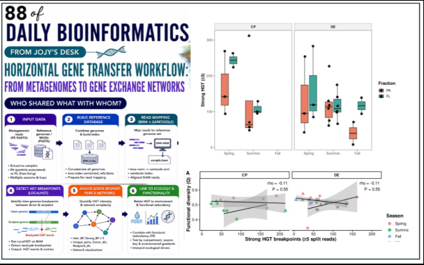
The dataset integrates HGT metrics, functional redundancy metrics, and environmental metadata across estuarine microbial communities sampled across two bays (Chesapeake and Delaware), three seasons (Spring, Summer, Fall), and two size fractions:
- Particle-associated (PA): microbes attached to particulate matter — physically aggregated, in close contact with each other
- Free-living (FL): microbes in the water column — dispersed, more exposed to environmental fluctuation
The key functional redundancy metric is R* (R-star): the realized functional redundancy of a community — a measure of how many taxa in the community can perform the same functional role. High R* means many taxa share the same functions; low R* means functions are partitioned uniquely across taxa. The core hypothesis going into this analysis was that communities with higher R* would show higher HGT — gene exchange as a mechanism for maintaining shared functional capacity across taxa.
Data preparation
library(tidyverse)
library(janitor)

df <- read_csv("HGT_fred.csv") %>%
  clean_names() %>%
  mutate(
    Season   = factor(season,   levels = c("Spring", "Summer", "Fall")),
    Fraction = factor(fraction, levels = c("PA", "FL"),
                      labels = c("Particle-associated", "Free-living")),
    Bay      = ifelse(bay == "CP", "Chesapeake", "Delaware"),
    # Resolve duplicate salinity columns if present
    salinity_num = as.numeric(salinity_5)
  )
janitor::clean_names() standardizes column names to lowercase with underscores — a one-line fix for the mixed-case, space-containing column names that come out of many summary tools. Before any analysis, confirm there are no duplicate columns (a common issue when merging summary files from different tools), and verify that all categorical variables have the levels you expect.
Core analysis: HGT and functional redundancy
Correlation between HGT and R*
# Spearman correlation — appropriate for non-normally distributed ecological data
cor.test(df$inter_bp,     df$rstar, method = "spearman")
cor.test(df$strong_bp_5,  df$rstar, method = "spearman")
cor.test(df$unique_pairs, df$rstar, method = "spearman")
Scatter plots
# HGT intensity vs functional redundancy
ggplot(df, aes(x = rstar, y = inter_bp, color = Fraction, shape = Bay)) +
  geom_point(size = 3, alpha = 0.8) +
  geom_smooth(method = "lm", se = TRUE, color = "black", linewidth = 0.7) +
  theme_bw(base_size = 13) +
  labs(
    x = "R* (Functional Redundancy)",
    y = "Inter-genome HGT breakpoints",
    title = "HGT intensity vs functional redundancy"
  )

# High-confidence HGT vs R*
ggplot(df, aes(x = rstar, y = strong_bp_5, color = Fraction, shape = Bay)) +
  geom_point(size = 3, alpha = 0.8) +
  geom_smooth(method = "lm", se = TRUE, color = "black", linewidth = 0.7) +
  theme_bw(base_size = 13) +
  labs(
    x = "R*",
    y = "Strong HGT breakpoints (≥5 reads)",
    title = "High-confidence HGT vs functional redundancy"
  )

# Network complexity vs R*
ggplot(df, aes(x = rstar, y = unique_pairs, color = Season, shape = Fraction)) +
  geom_point(size = 3, alpha = 0.8) +
  geom_smooth(method = "lm", se = TRUE, color = "black", linewidth = 0.7) +
  theme_bw(base_size = 13) +
  labs(
    x = "R*",
    y = "Unique donor–recipient pairs",
    title = "HGT network complexity vs functional redundancy"
  )
Linear models
# Main model: does HGT explain R* after accounting for ecology?
m1 <- lm(rstar ~ strong_bp_3 + bay + season + fraction + salinity_num, data = df)
summary(m1)

# Interaction: does the HGT–R* relationship differ by fraction?
m2 <- lm(inter_bp ~ rstar * Fraction + Season + Bay, data = df)
summary(m2)

# Partial correlation: does HGT–R* hold after controlling for environment?
library(ppcor)
pcor.test(df$inter_bp, df$rstar,
          df[, c("salinity_num", "temperature", "season_num")],
          method = "spearman")
Ecological patterns in HGT
Particle-associated vs. free-living
# Wilcoxon test: HGT differs by fraction?
wilcox_result <- df %>%
  group_by(Bay) %>%
  summarise(
    p_value    = wilcox.test(inter_bp[Fraction == "Particle-associated"],
                             inter_bp[Fraction == "Free-living"])$p.value,
    .groups = "drop"
  )

# Boxplot
ggplot(df, aes(x = Fraction, y = inter_bp, fill = Fraction)) +
  geom_boxplot(outlier.shape = NA) +
  geom_jitter(width = 0.15, alpha = 0.6, size = 2) +
  facet_wrap(~Bay) +
  theme_bw(base_size = 13) +
  labs(
    x = NULL, y = "Inter-genome HGT breakpoints",
    title = "HGT intensity by ecological compartment"
  )
Seasonal variation
ggplot(df, aes(x = Season, y = inter_bp, fill = Season)) +
  geom_boxplot(outlier.shape = NA) +
  geom_jitter(width = 0.1, alpha = 0.6, size = 2) +
  facet_wrap(~Fraction) +
  theme_bw(base_size = 13) +
  labs(x = NULL, y = "Inter-genome HGT breakpoints")
Environmental drivers
ggplot(df, aes(x = temperature, y = inter_bp, color = Fraction)) +
  geom_point(size = 3, alpha = 0.8) +
  geom_smooth(method = "lm", se = TRUE) +
  theme_bw(base_size = 13) +
  labs(x = "Temperature (°C)", y = "Inter-genome HGT breakpoints")
What the data actually showed
I want to be transparent about what this analysis found, because the result was not what the initial hypothesis predicted — and that is worth documenting.
The original hypothesis was that R* and HGT would be positively correlated: communities with more functional redundancy would show more gene exchange, because HGT is a mechanism for spreading functional traits across taxa.
What the data showed was that the relationship between HGT and R* was weak and non-significant across all tested metrics and stratifications. The correlations were small (ρ in the range of -0.18 to +0.13) and did not survive correction for multiple testing.
What did explain variation in the data was ecological compartment. Fraction (particle-associated vs. free-living) emerged as the dominant driver of both R* and HGT — but the two variables responded differently to it:
- R* was higher in particle-associated communities
- HGT was higher in free-living communities
This is a counterintuitive result for HGT. The conventional expectation is that physical proximity — which particle attachment provides — should promote gene transfer. The data suggests instead that free-living communities, which experience greater environmental variability and osmotic stress, may have stronger selective pressure for gene acquisition.
The revised conceptual model:
Environment (salinity, temperature, season)
        ↓                    ↓
    HGT patterns       Functional redundancy
Rather than HGT → R*, both HGT and R* are independently structured by the same environmental drivers. Whether HGT plays an indirect, lagged, or context-dependent role in shaping functional redundancy remains an open question — one that a time-series dataset, or a metatranscriptomic analysis of HGT-associated gene expression, could help answer.
Other tools for HGT detection in metagenomes
LocalHGT is one of several approaches for detecting HGT from metagenomic data. The right tool depends on whether you have isolate genomes, assembled MAGs, or only reads — and whether you want breakpoint-level evidence, phylogenetic incongruence, or both.
MetaCHIP
MetaCHIP detects HGT from assembled metagenomic bins (MAGs) by combining phylogenetic incongruence with best-match genome comparisons. For each gene in each MAG, it asks: does this gene cluster phylogenetically with genes from a distantly related organism? If so, it flags a candidate HGT event.
When to use it: You have high-quality MAGs and want to identify specific transferred genes and their likely donors, rather than just quantifying transfer intensity.
# Install
conda create -n metacchip -c bioconda -c conda-forge metacchip
conda activate metacchip

# Run
MetaCHIP PI -p project_name -r reference_genomes/ -g MAGs/ -t 16
MetaCHIP BP -p project_name
Output: a table of predicted HGT events with donor and recipient MAG assignments, gene identities, and confidence scores.
HGTector
HGTector uses a taxon-based approach: for each protein in a genome, it performs a sequence similarity search and asks whether the best matches are from the same taxonomic group as the query genome. Proteins that match organisms from distant phylogenetic groups are flagged as potential HGT acquisitions.
When to use it: You have isolate genomes or high-completeness MAGs and want to characterize the historical HGT landscape — which genes were acquired from which lineages — rather than detect active transfer events in a community.
# Install
conda create -n hgtector -c bioconda -c conda-forge hgtector
conda activate hgtector

# Search step (DIAMOND against NCBI nr)
hgtector search -i proteins.faa -o search_results/ -m diamond -db nr_db/

# Analyze step
hgtector analyze -i search_results/ -o hgtector_output/ -t taxonomy/
Output: scored protein list with HGT probability, donor group predictions, and summary statistics.
anvi’o pan-genomic HGT signals
anvi’o does not have a dedicated HGT detection module, but its pangenome framework can surface HGT signals indirectly. Gene clusters that are present in phylogenetically distant genomes within a pangenome — unexpected by vertical inheritance — are candidate HGT events. The anvi’o visualization interface allows you to inspect these directly, coloring the pangenome by phylogeny and manually identifying phylogenetically incongruent gene clusters.
When to use it: You are already running an anvi’o pangenome analysis and want to explore HGT in the context of the full accessory genome, without running a separate HGT-specific pipeline.
# After building the pangenome (see pangenomics post)
anvi-display-pan \
    -g GENOMES.db \
    -p pan_output/PAN.db \
    --server-only
In the browser interface, layer a phylogenetic tree alongside the gene cluster presence–absence matrix. Gene clusters that appear in isolated, phylogenetically distant branches of the tree, without intermediate occurrences, are visually apparent as HGT candidates.
Comparison summary
| Tool | Input | Approach | Best for |
|---|---|---|---|
| LocalHGT | Reads + reference genomes | Breakpoint detection | Quantifying active HGT in complex communities |
| MetaCHIP | MAGs / assembled bins | Phylogenetic incongruence | Identifying specific transferred genes between MAGs |
| HGTector | Isolate genomes or MAGs | Similarity-based taxonomy | Historical HGT characterization, donor identification |
| anvi’o | MAGs + pangenome | Visual incongruence inspection | Exploratory, in context of pangenome analysis |
In practice, these tools are complementary rather than competing. LocalHGT quantifies transfer intensity across a community at the read level. MetaCHIP or HGTector then identify which specific genes were transferred and from where. anvi’o ties everything together in the context of the pangenome.
Reproducibility checklist
- All LocalHGT runs use the same reference genome set — adding or removing reference genomes changes breakpoint counts and comparisons are only valid within a consistent reference.
- BAM files are sorted and indexed before LocalHGT input.
-
Strong_BP >= 5threshold is applied consistently and documented — the choice of cutoff affects how many events are retained. - Spearman correlation is used rather than Pearson for non-normally distributed ecological data.
- Multiple testing correction applied to Wilcoxon tests across seasons and fraction comparisons.
- Partial correlations computed to disentangle environmental confounders before interpreting HGT–R* relationships.
-
sessionInfo()saved alongside all R output.
sessionInfo()
Next steps
The analysis described here is cross-sectional: one timepoint per sample, one set of ecological variables. Several extensions would substantially strengthen the biological interpretation:
- Metatranscriptomic integration: Do HGT-associated genes show elevated expression in particle-associated communities despite lower transfer rates? This would separate acquisition from utilization.
- Pathway mapping: Which metabolic functions are being transferred? Mapping breakpoint-flanking genes to KEGG or CAZy pathways would reveal whether HGT is preferentially moving carbon cycling, nutrient cycling, or other ecologically relevant functions.
- Donor–recipient network visualization: The
Unique_pairsmetric summarizes network complexity as a single number. Building and visualizing the actual donor–recipient network in Cytoscape or igraph would reveal whether HGT is concentrated between a few highly connected hubs or distributed broadly across the community. - Time-series analysis: If samples span multiple years, does HGT intensity at time t predict changes in R* at time t+1? This lagged analysis is the most direct test of whether HGT shapes functional redundancy over time.
LocalHGT: github.com/songweizhi/LocalHGT. MetaCHIP: Songweizhi et al. (2020). HGTector: Zhu et al. (2014). Analysis performed on estuarine metatranscriptomic and metagenomic data across Chesapeake Bay and Delaware Bay sampling stations.