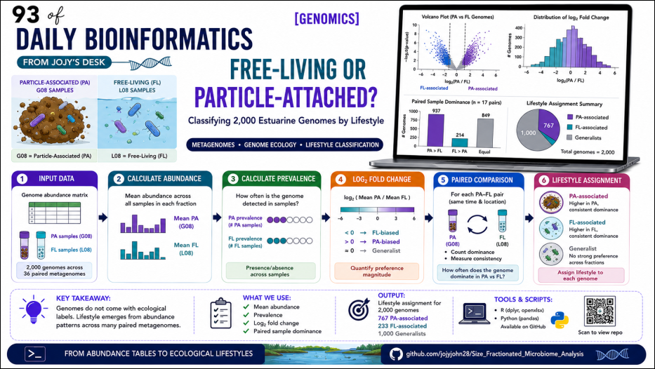
Free-living or Particle-attached? Classifying 2,000 Estuarine Genomes by Lifestyle from Paired Metagenomes

You ran a metagenome from a size-fractionated water sample. The particle-associated (PA) fraction — everything retained on a larger filter — went into one library. The free-living (FL) fraction — the smaller cells that passed through — went into another. You assembled, binned, and dereplicated everything into about 2,000 representative genomes. Now you want to know: which of these genomes actually belongs to the particle-associated lifestyle, and which is free-living?

The genomes themselves do not carry a label. A genome binned from a PA library might be from an organism that is genuinely PA-adapted — anchored to particles, producing extracellular enzymes — or it might just be a free-living organism that happened to be captured in the PA fraction that day. The way to separate these is not to look at where the genome came from during assembly. It is to look at how the genome’s abundance behaves across many samples: does it consistently show up at higher levels in PA fractions, or FL fractions, or does it not care?

This post documents exactly that classification workflow, applied to a dataset of 2,000 genomes across 36 paired PA/FL metagenomes from Chesapeake and Delaware Bay. The output — a lifestyle assignment for each genome — feeds directly into downstream functional comparisons of genome size, CAZyme content, and transporter repertoires.

All scripts are in the companion repository

The core logic

For each genome, we have an abundance value in every sample. Samples come in matched PA-FL pairs: CP_Spr01G08 (PA) and CP_Spr01L08 (FL) are the two fractions of the same water sample collected at the same time and location.

The classification uses three complementary metrics:

1. Mean abundance comparison — Is the average abundance across all PA samples higher than the average across all FL samples?

2. Log₂ fold-change — How large is the difference? log₂(mean_PA / mean_FL) > 0 means PA-biased; < 0 means FL-biased.

3. Paired dominance count — In how many matched pairs was this genome more abundant in the PA sample than in the FL sample from the same collection event? This accounts for the temporal and spatial structure of the sampling design.

Together these metrics tell you not just which fraction a genome prefers on average, but how consistently it expresses that preference across independent sampling events.

Sample naming convention

CP_Spr01G08  →  G08 suffix = Particle-Associated (PA)
CP_Spr01L08  →  L08 suffix = Free-Living (FL)

The base before the suffix (CP_Spr01) identifies the matched pair. This base-name extraction is how the pairing is done programmatically.

Input file

The abundance table is an Excel file with:

• Genome — genome identifier (matching the genome FASTA filename without extension)
• Genome_size_Mbp — total genome size in megabases
• Num_contigs — number of contigs in the assembly
• One column per sample — relative abundance values from CoverM

| Genome           | Genome_size_Mbp | Num_contigs | CP_Spr01G08 | CP_Spr01L08 | ... |
|------------------|-----------------|-------------|-------------|-------------|-----|
| GB_GCA_000153445 | 2.14            | 32          | 0.0012      | 0.0001      | ... |
| GB_GCA_000153745 | 1.81            | 19          | 0.0001      | 0.0045      | ... |

R workflow

Libraries

library(readxl)
library(dplyr)
library(openxlsx)

Step 1 — Read the abundance table

df <- read_excel(
  "Abd_updated_new.xlsx"
)

# Identify PA and FL sample columns by suffix
pa_cols <- grep("G08$", names(df), value = TRUE)
fl_cols <- grep("L08$", names(df), value = TRUE)

cat("PA columns:", length(pa_cols), "\n")   # 19
cat("FL columns:", length(fl_cols), "\n")   # 17

The dataset has 19 PA columns and 17 FL columns. This is common: not every PA sample has a surviving FL library and vice versa. The unequal column count does not prevent the mean calculation — rowMeans() handles it cleanly — but it does mean that only 17 matched pairs exist for the paired dominance analysis.

Step 2 — Mean abundance, prevalence, and log₂ fold-change

df2 <- df %>%
  mutate(
    # Mean abundance across all samples in each fraction
    Mean_PA = rowMeans(select(., all_of(pa_cols)), na.rm = TRUE),
    Mean_FL = rowMeans(select(., all_of(fl_cols)), na.rm = TRUE),

    # Prevalence: how many samples was this genome detected in?
    Prev_PA = rowSums(select(., all_of(pa_cols)) > 0, na.rm = TRUE),
    Prev_FL = rowSums(select(., all_of(fl_cols)) > 0, na.rm = TRUE),

    Total_Prev = Prev_PA + Prev_FL,

    # Log2 fold-change: positive = PA-biased, negative = FL-biased
    # Pseudocount prevents log(0)
    log2_PA_FL = log2((Mean_PA + 1e-9) / (Mean_FL + 1e-9))
  )

The pseudocount 1e-9 is small enough to be negligible for genomes with real signal, but prevents log(0/0) = NaN for genomes that were absent from one fraction entirely.

Important distinction: Prev_PA = 19 does not mean the genome was more abundant in PA than FL in 19 samples. It means it was detected (abundance > 0) in 19 PA samples. A genome could be detected in all PA samples but still have higher FL abundance in most of them. The paired dominance count in Step 4 is what captures actual directional dominance.

Step 3 — Lifestyle classification

df2 <- df2 %>%
  mutate(
    Lifestyle = case_when(
      Mean_PA > Mean_FL ~ "PA_associated",
      Mean_FL > Mean_PA ~ "FL_associated",
      TRUE              ~ "Equal"
    )
  )

table(df2$Lifestyle)

FL_associated   PA_associated
          233             767

767 genomes show higher average abundance in the PA fraction; 233 show higher average abundance in FL. The PA-heavy skew reflects the composition of the sampling design — PA filters capture a larger and more diverse biomass than the FL fraction in most estuarine environments.

Step 4 — Paired dominance analysis

This step asks: in matched sample pairs, how consistently does this genome favour one fraction?

# Match PA and FL columns by base name
pa_base     <- sub("G08$", "", pa_cols)
fl_base     <- sub("L08$", "", fl_cols)
common_base <- intersect(pa_base, fl_base)

cat("Matched pairs:", length(common_base), "\n")   # 17

matched_pa_cols <- paste0(common_base, "G08")
matched_fl_cols <- paste0(common_base, "L08")

# Initialise counters
df2$PA_Higher_Count <- 0
df2$FL_Higher_Count <- 0
df2$Equal_Count     <- 0

for (i in seq_along(matched_pa_cols)) {
  pa_vec <- df2[[matched_pa_cols[i]]]
  fl_vec <- df2[[matched_fl_cols[i]]]

  df2$PA_Higher_Count <- df2$PA_Higher_Count + as.integer(pa_vec > fl_vec)
  df2$FL_Higher_Count <- df2$FL_Higher_Count + as.integer(fl_vec > pa_vec)
  df2$Equal_Count     <- df2$Equal_Count     + as.integer(pa_vec == fl_vec)
}

df2$Total_Paired_Comparisons <- df2$PA_Higher_Count + df2$FL_Higher_Count + df2$Equal_Count

df2$PA_Dominance_Percent <-
  100 * df2$PA_Higher_Count / df2$Total_Paired_Comparisons

df2$FL_Dominance_Percent <-
  100 * df2$FL_Higher_Count / df2$Total_Paired_Comparisons

A genome with PA_Higher_Count = 15 out of 17 pairs (88%) is reliably PA-associated across the full temporal and spatial range of the dataset. A genome with PA_Higher_Count = 9 out of 17 (53%) is barely tilted toward PA — its lifestyle classification is much less confident.

This paired dominance metric is the one to report alongside the mean-based Lifestyle column when describing individual genomes of interest in the manuscript.

Step 5 — Save outputs

# Full table with all new columns
write.xlsx(
  df2,
  "Abd_updated_new_with_lifestyle.xlsx",
  overwrite = TRUE
)

write.csv(df2, "Abd_updated_new_with_lifestyle.csv", row.names = FALSE)

# Reduced metadata file — for merging with CAZyme and transporter results
metadata_df <- df2 %>%
  select(
    Genome, Genome_size_Mbp, Num_contigs,
    Mean_PA, Mean_FL, Prev_PA, Prev_FL, Total_Prev,
    log2_PA_FL, Lifestyle,
    PA_Higher_Count, FL_Higher_Count, Equal_Count,
    Total_Paired_Comparisons, PA_Dominance_Percent, FL_Dominance_Percent
  )

write.csv(metadata_df, "genome_metadata_lifestyle.csv", row.names = FALSE)

Merging lifestyle assignments with functional annotations (Python)

Once lifestyle assignments exist in genome_metadata_lifestyle.csv, they need to be joined with CAZyme counts (from dbCAN) and transporter counts (from TCDB DIAMOND hits). Python pandas handles this cleanly.

Merge CAZyme counts with lifestyle

import pandas as pd

# Load feature table (CAZyme counts per genome)
cazy = pd.read_excel('cazy_genome.xlsx')

# Load lifestyle reference
lifestyle = pd.read_excel('life_style_reference.xlsx')

# Clean column names and IDs — essential step
cazy.columns      = cazy.columns.str.strip()
lifestyle.columns = lifestyle.columns.str.strip()

# IDs must be strings — Excel sometimes reads genome accessions as floats
cazy['Genome']      = cazy['Genome'].astype(str).str.strip()
lifestyle['Genome'] = lifestyle['Genome'].astype(str).str.strip()

# Merge on Genome ID
merged = pd.merge(cazy, lifestyle, on='Genome', how='left', indicator=True)

# Check how many matched
print(merged['_merge'].value_counts())

# Keep matched rows only
matched = merged[merged['_merge'] == 'both'].drop(columns='_merge')

matched.to_excel('CAZy_with_lifestyle.xlsx', index=False)
print(f"Saved {len(matched)} genomes with lifestyle annotations.")

Merge transporter counts with lifestyle

The same pattern applies to transporter counts. The transporter file (transporters.tsv) has one row per genome with summarized counts per TCDB family:

# Load transporter summary (from DIAMOND TCDB hits, summarized per genome)
transporters = pd.read_csv('transporters.tsv', sep='\t')
lifestyle     = pd.read_csv('genome_metadata_lifestyle.csv')

# Clean IDs
transporters['Genome'] = transporters['Genome'].astype(str).str.strip()
lifestyle['Genome']    = lifestyle['Genome'].astype(str).str.strip()

# Merge
transport_lifestyle = pd.merge(
    transporters, lifestyle[['Genome', 'Lifestyle', 'log2_PA_FL',
                              'PA_Dominance_Percent', 'Genome_size_Mbp']],
    on='Genome', how='left'
)

# Save
transport_lifestyle.to_csv('transporters_with_lifestyle.csv', index=False)

# Quick summary: mean ABC transporter count by lifestyle
print(
    transport_lifestyle.groupby('Lifestyle')['ABC_gene_count'].describe()
)

The indicator=True + _merge check is the pandas equivalent of R’s alignment check — always run it. If many rows are left_only (present in the feature table but not in the lifestyle reference), it means there is an ID mismatch that needs tracing before proceeding.

Common ID mismatch causes

# Diagnose mismatches: find IDs in CAZy table not in lifestyle reference
unmatched = cazy[~cazy['Genome'].isin(lifestyle['Genome'])]
print(f"{len(unmatched)} genomes in CAZy not found in lifestyle reference")
print(unmatched['Genome'].head(10))

# Common causes:
# 1. Trailing whitespace — fixed by .str.strip() above
# 2. Version suffix mismatch: "GB_GCA_000153445.1" vs "GB_GCA_000153445"
#    Fix: strip version
cazy['Genome']      = cazy['Genome'].str.replace(r'\.\d+$', '', regex=True)
lifestyle['Genome'] = lifestyle['Genome'].str.replace(r'\.\d+$', '', regex=True)

# 3. Excel float conversion: "1234567.0" instead of "1234567"
#    Fix: convert to int first
cazy['Genome'] = cazy['Genome'].str.replace(r'\.0$', '', regex=True)

What the output looks like

From the images above, the final merged table has:

• Each genome in its own row with the lifestyle assignment (PA_associated or FL_associated)
• Genome name in GTDB format (e.g., s__Luminipleurotus → cyanobacteria, s__HIMB30 → SAR11, a canonical free-living marine oligotroph)
• Functional counts (ABC transporter gene count, CAZyme family counts) alongside the lifestyle label

This table is the input to every downstream statistical comparison: Wilcoxon tests comparing genome size, total GH count, TBDT count, and ABC transporter count between PA and FL lifestyle groups.

Output columns reference

This analysis is still on going , so changes in the workflow can be expected.