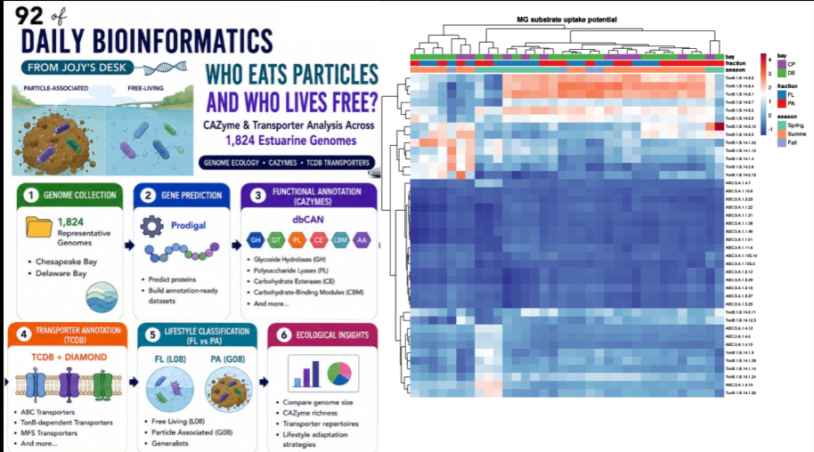
Who Eats Particles and Who Lives Free? CAZyme and Transporter Analysis Across 1,824 Estuarine Genomes
A particle of organic matter sinking through an estuary is not just food — it is a habitat. Bacteria that colonize it can anchor themselves to a surface enriched in polymers, produce extracellular enzymes to break those polymers down, and capture the liberated sugars and amino acids through specialized transporters. The free-living bacterium suspended in the water column next to them faces a completely different challenge: the dissolved organic matter it depends on is dilute, chemically diverse, and constantly changing. These two lifestyles impose different selective pressures on genome content.
This post documents an ongoing analysis of 1,824 representative estuarine genomes — annotating their carbohydrate-active enzymes (CAZymes) with dbCAN and their transport systems with the TCDB database, then linking those functional profiles to observed free-living (FL) vs particle-associated (PA) abundance patterns. The hypothesis is simple: PA-associated genomes should carry more and different CAZymes, more polymer-degrading machinery, and more specialized transport systems. FL-associated genomes should be more streamlined. Whether the data supports this is what the analysis will show.
All scripts are available in the companion GitHub repository (link below) and will be updated as the analysis progresses.
Background: why CAZymes and transporters?
CAZymes — carbohydrate-active enzymes
Carbohydrates are the most abundant class of organic molecules in marine and estuarine systems. Polysaccharides from phytoplankton cell walls, terrestrial plant material, and microbial biomass make up the bulk of particulate organic carbon. Bacteria that can degrade these polymers occupy a critical ecological position.
CAZymes are classified by the CAZy database into functional families:
| Class | Full name | What it does |
|---|---|---|
| GH | Glycoside Hydrolases | Cleave glycosidic bonds — the primary polymer degraders |
| GT | Glycosyltransferases | Build glycosidic bonds — cell wall and EPS synthesis |
| PL | Polysaccharide Lyases | Cleave uronic acid-containing polymers (alginate, pectin) |
| CE | Carbohydrate Esterases | Remove ester substituents from polysaccharides |
| AA | Auxiliary Activities | Oxidative enzymes supporting degradation |
| CBM | Carbohydrate-Binding Modules | Bind substrate without catalysis — target enzymes to substrate |
A genome with many GH and PL families is equipped for complex polymer degradation. A genome with few GH but many GT is more focused on cell wall maintenance than substrate acquisition.
Transporters — TCDB
Once a polymer is cleaved into oligosaccharides or monomers, those substrates need to enter the cell. The Transporter Classification Database (TCDB) classifies membrane transport systems by mechanism and substrate range. In the context of FL vs PA ecology, three families are particularly informative:
- ABC transporters — ATP-powered, high-affinity uptake. Excellent for capturing substrates at low concentrations — the free-living niche
- TBDTs (TonB-dependent transporters) — outer membrane proteins specialized for capturing large oligosaccharides. Associated with particle degradation in marine bacteria
- MFS transporters — major facilitator superfamily; broad substrate range, important in both niches
The prediction is that PA genomes will be enriched in TBDTs (polymer product capture) while FL genomes will be enriched in high-affinity ABC transporters for dissolved substrates.
Dataset
- 1,824 representative estuarine MAGs/genomes from Chesapeake Bay and Delaware Bay samples
- Selected as the top 2,000 quality genomes from a larger assembly; 1,824 passed annotation quality checks
- 30 samples (metagenomes) providing relative abundance data: G08 = Particle-Associated, L08 = Free-Living
Project structure
CAZyme_TCDB_genomes/
├── 00_lists/
│   ├── genomes_fasta.list          # one genome path per line
│   └── annotated_1824_genomes.txt  # genome IDs for abundance extraction
├── 01_proteins/                    # Prodigal protein predictions per genome
├── 02_dbcan/                       # dbCAN output per genome
├── 03_tcdb/                        # DIAMOND TCDB results per genome
└── scripts/                        # all analysis scripts (GitHub repo)
Scripts repository: github.com/JojyJohn/Fl_vs_PA_genome_analysis (updating as analysis progresses)
Step 1 — Build the genome list
# 00_make_genome_list.sh
find genomes_top2000/genomes_fasta -name "*.fna" \
  | sort > 00_lists/genomes_fasta.list

wc -l 00_lists/genomes_fasta.list   # should be 1824
A flat text file with one genome path per line is the input to every downstream SLURM array job. Line number N in the file corresponds to SLURM_ARRAY_TASK_ID=N, so the array index directly selects the genome to process.
Step 2 — Protein prediction with Prodigal
Before annotating functions, we need protein sequences. Prodigal predicts protein-coding genes from assembled genome sequences using a dynamic programming model of prokaryotic gene structure.
# 01_predict_proteins_prodigal.sh
#!/bin/bash
#SBATCH --job-name=prodigal_genomes
#SBATCH --cpus-per-task=4
#SBATCH --mem=20G
#SBATCH --time=04:00:00
#SBATCH --array=1-1824%50

module load prodigal

BASE=/project/bcampb7/camplab/Jojy/Fl_vs_PA_2026_Jojy/CAZyme_TCDB_genomes
LIST=${BASE}/00_lists/genomes_fasta.list

GENOME=$(sed -n "${SLURM_ARRAY_TASK_ID}p" ${LIST})
GENOME_ID=$(basename ${GENOME} .fna)
OUTDIR=${BASE}/01_proteins/${GENOME_ID}

mkdir -p ${OUTDIR}

prodigal \
  -i ${GENOME} \
  -a ${OUTDIR}/${GENOME_ID}.faa \   # amino acid sequences → input to dbCAN and DIAMOND
  -d ${OUTDIR}/${GENOME_ID}.ffn \   # nucleotide sequences
  -o ${OUTDIR}/${GENOME_ID}.gff \   # gene coordinates
  -p meta                            # metagenome mode
-p meta is important: standard Prodigal mode trains a gene model on the input sequence, which works well for complete genomes but fails for short or fragmented MAG contigs. Metagenome mode uses pre-trained models and is appropriate for assemblies of any size or completeness.
The %50 in --array=1-1824%50 limits simultaneous jobs to 50 — a cluster-polite way to process 1,824 genomes without monopolizing the queue.
Output per genome:
-
.faa— protein sequences (input to all downstream annotation) -
.ffn— nucleotide CDS sequences -
.gff— gene coordinates
Step 3 — CAZyme annotation with dbCAN
dbCAN annotates CAZymes using a curated HMM database built from the CAZy family definitions. We use the HMMER tool only (--tools hmmer) for speed and reliability.
# 02_run_dbcan_genomes.sh
#!/bin/bash
#SBATCH --job-name=dbcan_genomes
#SBATCH --cpus-per-task=16
#SBATCH --mem=100G
#SBATCH --time=24:00:00
#SBATCH --array=1-1824%20

conda activate dbcan

BASE=/project/bcampb7/camplab/Jojy/Fl_vs_PA_2026_Jojy/CAZyme_TCDB_genomes
DBCAN_DB=/project/bcampb7/camplab/Jojy/Fl_vs_PA_2026_Jojy/databases/dbcan
LIST=${BASE}/00_lists/genomes_fasta.list

GENOME=$(sed -n "${SLURM_ARRAY_TASK_ID}p" ${LIST})
GENOME_ID=$(basename ${GENOME} .fna)

PROTEINS=${BASE}/01_proteins/${GENOME_ID}/${GENOME_ID}.faa
OUTDIR=${BASE}/02_dbcan/${GENOME_ID}

mkdir -p ${OUTDIR}

run_dbcan \
  ${PROTEINS} protein \
  --out_dir ${OUTDIR} \
  --db_dir ${DBCAN_DB} \
  --dbCANFile ${DBCAN_DB}/dbCAN-HMMdb-V14.txt \
  --hmm_cpu 16 \
  --tools hmmer
Key output file: overview.txt — one row per predicted CAZyme, with the protein ID, CAZyme family, and E-value. This is what gets concatenated across all 1,824 genomes in Step 6.
Step 4 — Transporter annotation with TCDB + DIAMOND
The TCDB database does not have a dedicated annotation tool like dbCAN. Instead, we perform a sequence similarity search using DIAMOND blastp against the TCDB protein database.
# 03_run_tcdb_genomes.sh
#!/bin/bash
#SBATCH --job-name=tcdb_genomes
#SBATCH --cpus-per-task=16
#SBATCH --mem=100G
#SBATCH --time=12:00:00
#SBATCH --array=1-1824%30

module load diamond

BASE=/project/bcampb7/camplab/Jojy/Fl_vs_PA_2026_Jojy/CAZyme_TCDB_genomes
TCDB_DB=/project/bcampb7/camplab/Jojy/Fl_vs_PA_2026_Jojy/databases/tcdb/tcdb
LIST=${BASE}/00_lists/genomes_fasta.list

GENOME=$(sed -n "${SLURM_ARRAY_TASK_ID}p" ${LIST})
GENOME_ID=$(basename ${GENOME} .fna)

PROTEINS=${BASE}/01_proteins/${GENOME_ID}/${GENOME_ID}.faa
OUTDIR=${BASE}/03_tcdb

mkdir -p ${OUTDIR}

diamond blastp \
  --db ${TCDB_DB} \
  --query ${PROTEINS} \
  --out ${OUTDIR}/${GENOME_ID}_tcdb.tsv \
  --outfmt 6 qseqid sseqid pident length mismatch gapopen qstart qend sstart send evalue bitscore stitle \
  --evalue 1e-5 \
  --query-cover 50 \
  --subject-cover 50 \
  --threads 16 \
  --sensitive
Filtering thresholds: --evalue 1e-5, --query-cover 50, --subject-cover 50 are conservative but standard for functional annotation. The bidirectional coverage filter (query and subject must each have ≥50% coverage) reduces false positives from partial domain matches.
The stitle field in the output captures the TCDB subject title, which encodes the transporter family classification. This is parsed downstream to assign each hit to a TCDB family class.
Step 5 — FL vs PA genome classification
Extract abundance for the 1,824 annotated genomes
The full abundance table covers 25,838 genomes. We extract only the 1,824 that passed annotation:
# extract_1824_abundance_and_classify.py
import pandas as pd

# Load full abundance table
abund = pd.read_csv("genome_abundance_table_approachA.tsv", sep="\t", index_col=0)

# Load the list of annotated genomes
genome_list = pd.read_csv("00_lists/annotated_1824_genomes.txt", header=None, names=["genome"])

# Filter to annotated genomes only
abund_1824 = abund.loc[abund.index.isin(genome_list["genome"])]

print(f"Retained {len(abund_1824)} genomes from {len(abund)} total")

# Identify PA and FL samples by naming convention
pa_cols = [c for c in abund_1824.columns if "G08" in c]   # Particle-associated
fl_cols = [c for c in abund_1824.columns if "L08" in c]   # Free-living

# Calculate mean abundance per lifestyle
abund_1824["mean_PA"] = abund_1824[pa_cols].mean(axis=1)
abund_1824["mean_FL"] = abund_1824[fl_cols].mean(axis=1)

# Log2 fold change: positive = PA-enriched, negative = FL-enriched
abund_1824["log2_PA_FL"] = (
    (abund_1824["mean_PA"] + 1e-10).apply(pd.np.log2) -
    (abund_1824["mean_FL"] + 1e-10).apply(pd.np.log2)
)

# Classify
def classify(log2fc):
    if log2fc > 1:
        return "PA-associated"
    elif log2fc < -1:
        return "FL-associated"
    else:
        return "Generalist"

abund_1824["lifestyle"] = abund_1824["log2_PA_FL"].apply(classify)

print(abund_1824["lifestyle"].value_counts())

abund_1824[["mean_PA", "mean_FL", "log2_PA_FL", "lifestyle"]].to_csv(
    "genome_lifestyle_classification.tsv", sep="\t"
)
Classification results
| Lifestyle | Genomes |
|---|---|
| Generalist | 1,233 |
| PA-associated | 337 |
| FL-associated | 254 |
| Total | 1,824 |
The majority of genomes are generalists — consistent with the ecological reality that most estuarine bacteria are not strictly confined to one lifestyle. The 337 PA-associated and 254 FL-associated genomes are the primary targets for functional comparison.
Step 6 — Concatenate annotation results
dbCAN
# concatenate_dbcan_tcdb.py (dbCAN section)
import pandas as pd
from pathlib import Path

dbcan_dir = Path("02_dbcan")
dfs = []

for file in dbcan_dir.glob("*/overview.txt"):
    genome = file.parent.name
    df = pd.read_csv(file, sep="\t")
    df.insert(0, "Genome", genome)
    dfs.append(df)

combined = pd.concat(dfs, ignore_index=True)
combined.to_csv("all_dbcan_overview_with_genome.tsv", sep="\t", index=False)

print(f"Total CAZyme annotations: {len(combined)}")
print(f"Genomes represented: {combined['Genome'].nunique()}")
TCDB
# concatenate_dbcan_tcdb.py (TCDB section)
cols = ["qseqid","sseqid","pident","length","mismatch","gapopen",
        "qstart","qend","sstart","send","evalue","bitscore","stitle"]

dfs = []
for file in Path("03_tcdb").glob("*_tcdb.tsv"):
    genome = file.name.replace("_tcdb.tsv", "")
    df = pd.read_csv(file, sep="\t", header=None, names=cols)
    df.insert(0, "Genome", genome)
    dfs.append(df)

combined_tcdb = pd.concat(dfs, ignore_index=True)
combined_tcdb.to_csv("all_tcdb_with_genome.tsv", sep="\t", index=False)
Step 7 — Genome size calculation
Genome size is expected to differ between FL and PA lifestyles — streamlined FL genomes vs. larger, more metabolically flexible PA genomes. We calculate it directly from the FASTA files:
# calculate_genome_sizes.py
from Bio import SeqIO
import os

results = []

for fasta in open("00_lists/genomes_fasta.list"):
    fasta = fasta.strip()
    genome = os.path.basename(fasta).replace(".fna", "")
    total_bp, contigs = 0, 0

    for record in SeqIO.parse(fasta, "fasta"):
        total_bp += len(record.seq)
        contigs += 1

    results.append({
        "Genome": genome,
        "Genome_size_bp": total_bp,
        "Genome_size_Mbp": round(total_bp / 1e6, 3),
        "Num_contigs": contigs
    })

import pandas as pd
pd.DataFrame(results).to_csv("genome_sizes.tsv", sep="\t", index=False)
Building the integrated analysis table
The final merged table brings together everything:
library(tidyverse)

lifestyle  <- read_tsv("genome_lifestyle_classification.tsv")
cazymes    <- read_tsv("all_dbcan_overview_with_genome.tsv")
tcdb       <- read_tsv("all_tcdb_with_genome.tsv")
sizes      <- read_tsv("genome_sizes.tsv")

# Summarize CAZyme counts per genome and family class
cazyme_counts <- cazymes %>%
  mutate(family_class = str_extract(HMMER, "^[A-Z]+")) %>%
  group_by(Genome, family_class) %>%
  summarise(count = n(), .groups = "drop") %>%
  pivot_wider(names_from = family_class, values_from = count, values_fill = 0)

# Summarize TCDB transporter family counts per genome
tcdb_counts <- tcdb %>%
  mutate(
    tcdb_class = str_extract(sseqid, "^[0-9]+\\.[A-Z]"),
    family = case_when(
      str_detect(stitle, "ABC")  ~ "ABC",
      str_detect(stitle, "TBDT|TonB") ~ "TBDT",
      str_detect(stitle, "MFS") ~ "MFS",
      TRUE ~ "Other"
    )
  ) %>%
  group_by(Genome, family) %>%
  summarise(count = n(), .groups = "drop") %>%
  pivot_wider(names_from = family, values_from = count, values_fill = 0)

# Merge all tables
integrated <- lifestyle %>%
  left_join(sizes,        by = "Genome") %>%
  left_join(cazyme_counts, by = "Genome") %>%
  left_join(tcdb_counts,   by = "Genome") %>%
  mutate(across(where(is.numeric), ~replace_na(.x, 0)))

write_tsv(integrated, "genome_integrated_FL_PA_analysis.tsv")
Planned statistical analyses
With the integrated table built, the comparisons of interest are:
library(rstatix)

# Kruskal-Wallis test across three lifestyle groups
# (non-parametric, appropriate for skewed count distributions)
kruskal_results <- integrated %>%
  pivot_longer(
    cols = c(Genome_size_Mbp, GH, GT, PL, CBM, AA, ABC, TBDT, MFS),
    names_to  = "metric",
    values_to = "value"
  ) %>%
  group_by(metric) %>%
  kruskal_test(value ~ lifestyle)

# Post-hoc pairwise Wilcoxon tests with BH correction
pairwise_results <- integrated %>%
  pivot_longer(
    cols = c(Genome_size_Mbp, GH, GT, PL, CBM, AA, ABC, TBDT, MFS),
    names_to = "metric", values_to = "value"
  ) %>%
  group_by(metric) %>%
  wilcox_test(value ~ lifestyle, p.adjust.method = "BH")
Biological hypotheses being tested
| Prediction | Direction | Metric |
|---|---|---|
| PA genomes have larger genomes | PA > FL | Genome_size_Mbp |
| PA genomes encode more CAZymes | PA > FL | GH, PL, CBM total |
| PA genomes are richer in polymer lyases | PA > FL | PL |
| PA genomes carry more TBDTs | PA > FL | TBDT |
| FL genomes are enriched in ABC transporters | FL > PA | ABC |
| Generalists intermediate | PA > Gen > FL | all metrics |
These are directional hypotheses — the analysis will test whether the data supports them, and document cases where it does not. The most interesting results are likely to be the exceptions: PA genomes without CAZyme enrichment, FL genomes with unexpectedly complex transport systems. Those outliers tell the most nuanced story about lifestyle flexibility in estuarine microbiomes.
Repository and reproducibility
Current scripts:
| Script | Purpose |
|---|---|
00_make_genome_list.sh | Generate sorted genome path list |
01_predict_proteins_prodigal.sh | SLURM array: Prodigal protein prediction |
02_run_dbcan_genomes.sh | SLURM array: dbCAN CAZyme annotation |
03_run_tcdb_genomes.sh | SLURM array: DIAMOND TCDB transporter search |
calculate_genome_sizes.py | Calculate genome size from FASTA |
concatenate_dbcan_tcdb.py | Merge per-genome annotation outputs |
extract_1824_abundance_and_classify.py | Extract abundance and classify FL/PA/Generalist |
run_dbcan_hmm_genome.sh | Single-genome dbCAN wrapper for testing |
The repository will be updated as downstream analyses (statistical comparisons, figures, integrated table generation) are completed. Please see 7th Day repo**
Analysis ongoing — results and scripts will be updated as the project progresses. dbCAN version: HMMdb-V14. TCDB accessed May 2026. Genome dataset: 1,824 representative MAGs from Chesapeake Bay and Delaware Bay estuarine metagenomes.