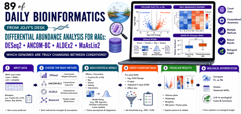
Differential Abundance Analysis for MAGs: DESeq2, ANCOM-BC, ALDEx2, and MaAsLin2
🧬 𝐷𝑎𝑦 𝟪9 𝑜𝑓 𝐷𝑎𝑖𝑙𝑦 𝐵𝑖𝑜𝑖𝑛𝑓𝑜𝑟𝑚𝑎𝑡𝑖𝑐𝑠 𝑓𝑟𝑜𝑚 𝐽𝑜𝑗𝑦’𝑠 𝖽𝖾𝗌𝗄
Community composition tells you who is there. A relative abundance table of 2,000 MAGs tells you, for each sample, what fraction of the sequencing signal each genome contributes. That is valuable — but it does not answer the question that usually matters most: which genomes are actually changing between my conditions? Which MAGs are consistently more abundant in particle-associated communities than free-living ones? Which respond to seasonal shifts? Which distinguish a disturbed estuary from a reference site?
That question belongs to differential abundance analysis. And in the world of metagenomics, choosing the right method for it is genuinely important — not just a technical nicety — because the nature of sequencing data breaks several assumptions that classical statistics rely on.
This post covers four methods: DESeq2, ANCOM-BC, ALDEx2, and MaAsLin2. For each one I explain what it does, when it is appropriate, and how to run it. I also show a real example from an estuarine FL vs PA dataset, document the most common mistakes, and give you a decision table for choosing which method to reach for given your data type and study design.
Why standard statistics fail on abundance data
Before getting into methods, it is worth understanding why a t-test or linear model on relative abundances is problematic. The issue is compositionality: in a sequencing experiment, you observe proportions, not absolute counts. If genome A increases in absolute abundance but everything else stays the same, its relative abundance goes up. But if genome B doubles, genome A’s relative abundance goes down — even though genome A did nothing. Every feature is coupled to every other feature through the constant-sum constraint.
A toy example:
| Genome | Sample 1 (absolute) | Sample 2 (absolute) | Sample 1 (relative) | Sample 2 (relative) |
|---|---|---|---|---|
| MAG_001 | 100 | 100 | 50% | 33% |
| MAG_002 | 50 | 100 | 25% | 33% |
| MAG_003 | 50 | 100 | 25% | 33% |
MAG_001 did not change at all in absolute terms. But its relative abundance dropped from 50% to 33% because MAG_002 and MAG_003 doubled. A naive differential test on relative abundances would flag MAG_001 as significantly decreased — a false positive driven entirely by compositional coupling.
Methods like ANCOM-BC and ALDEx2 are specifically designed to handle this. DESeq2, which operates on raw counts, sidesteps it differently. Understanding this distinction drives almost every decision in differential abundance analysis.
Input data: what you need
Regardless of method, you need two files:
1. Abundance table — MAGs as rows, samples as columns. The format varies by method:
           Sample_1   Sample_2   Sample_3   Sample_4
MAG_001      1240        880       2100        560
MAG_002       430        210        880        120
MAG_003         0         90        430         80
...
For DESeq2: raw integer read counts (from featureCounts, CoverM, or similar). For ANCOM-BC, ALDEx2, MaAsLin2: raw counts are preferred; relative abundances work for ALDEx2 and MaAsLin2 but raw counts are better when available.
2. Metadata — samples as rows, covariates as columns:
           Fraction   Bay          Season   Salinity
Sample_1   PA         Chesapeake   Spring   Low
Sample_2   FL         Chesapeake   Spring   Low
Sample_3   PA         Delaware     Summer   High
Sample_4   FL         Delaware     Summer   High
Before running any method, verify alignment:
all(colnames(counts) == rownames(metadata)) # must return TRUE
Method 1: DESeq2
DESeq2 was developed for RNA-seq and is the most widely used differential abundance method in genomics. It models count data using a negative binomial distribution — which handles the overdispersion typical in sequencing data better than a Poisson model — and uses a shrinkage estimator for fold-change to stabilize estimates for low-count features.
When to use it
DESeq2 is well suited for MAG differential abundance when you have raw read counts, a relatively balanced experimental design, and want well-characterized statistical behavior. It handles complex multi-factor designs cleanly and integrates well with the tidyverse visualization ecosystem.
Do not use DESeq2 on relative abundances. The negative binomial model requires integer counts. Feeding it proportions breaks the model silently — it will run and produce numbers, but those numbers are not statistically valid.
Installation
if (!require("BiocManager", quietly = TRUE))
    install.packages("BiocManager")
BiocManager::install("DESeq2")
Running DESeq2
library(DESeq2)
library(tidyverse)

# Load data
counts   <- read.csv("mag_counts.csv", row.names = 1, check.names = FALSE)
metadata <- read.csv("metadata.csv",   row.names = 1, check.names = FALSE)

# Verify alignment
stopifnot(all(colnames(counts) == rownames(metadata)))

# Set reference level explicitly
metadata$Fraction <- factor(metadata$Fraction, levels = c("PA", "FL"))

# Build DESeqDataSet
dds <- DESeqDataSetFromMatrix(
  countData = counts,
  colData   = metadata,
  design    = ~ Fraction        # adjust for additional factors: ~ Bay + Season + Fraction
)

# Optional: filter low-count MAGs before running
dds <- dds[rowSums(counts(dds) >= 10) >= 3, ]

# Run
dds <- DESeq(dds)
resultsNames(dds)   # always check contrast names before extracting

# Extract results
res <- results(dds, name = "Fraction_FL_vs_PA", alpha = 0.05)
res_df <- as.data.frame(res) %>%
  rownames_to_column("MAG") %>%
  arrange(padj)

# Significant MAGs
sig <- res_df %>%
  filter(padj < 0.05, abs(log2FoldChange) > 1)

write.csv(res_df, "DESeq2_FL_vs_PA_all.csv", row.names = FALSE)
write.csv(sig,    "DESeq2_FL_vs_PA_significant.csv", row.names = FALSE)
Volcano plot
library(ggrepel)

volcano_df <- res_df %>%
  filter(!is.na(padj), !is.na(log2FoldChange)) %>%
  mutate(
    significant = padj < 0.05 & abs(log2FoldChange) > 1,
    direction   = case_when(
      significant & log2FoldChange > 0 ~ "Enriched in FL",
      significant & log2FoldChange < 0 ~ "Enriched in PA",
      TRUE ~ "Not significant"
    )
  )

top_labels <- volcano_df %>%
  filter(significant) %>%
  slice_min(padj, n = 15)

ggplot(volcano_df, aes(x = log2FoldChange, y = -log10(padj))) +
  geom_point(aes(color = direction), alpha = 0.6, size = 1.8) +
  geom_text_repel(
    data = top_labels, aes(label = MAG),
    size = 2.8, max.overlaps = 20,
    box.padding = 0.3, segment.color = "grey60"
  ) +
  geom_vline(xintercept = c(-1, 1),  linetype = "dashed", linewidth = 0.4) +
  geom_hline(yintercept = -log10(0.05), linetype = "dashed", linewidth = 0.4) +
  scale_color_manual(values = c(
    "Enriched in FL"  = "#3182BD",
    "Enriched in PA"  = "#E6550D",
    "Not significant" = "grey75"
  )) +
  theme_bw(base_size = 13) +
  theme(
    panel.grid.minor = element_blank(),
    legend.position  = "bottom"
  ) +
  labs(
    x     = "Log2 Fold Change (FL vs PA)",
    y     = "-Log10 Adjusted P-value",
    color = NULL,
    title = "Differential MAG abundance: Free-living vs Particle-associated"
  )
Points to the right (positive log2FC) are enriched in FL; points to the left are enriched in PA. The dashed lines mark the significance threshold (horizontal) and the ±1 fold-change filter (vertical). Only points in the upper-left and upper-right quadrants — beyond both lines — are the confident, biologically relevant hits.
Method 2: ANCOM-BC (and ANCOM-BC2)
ANCOM-BC (Analysis of Compositions of Microbiomes with Bias Correction) was developed specifically for compositional microbiome data. Its key insight is that the observed log-ratio between two samples contains not just the true biological signal but also a sampling fraction bias — the fact that different samples were sequenced to different depths. ANCOM-BC estimates and removes this bias before testing for differences.
ANCOM-BC2 (the current recommended version) extends this with better handling of rare features, improved type I error control, and support for more complex study designs.
When to use it
ANCOM-BC is the right choice when you are concerned about compositional effects and want a method with strong theoretical grounding in the statistics of relative abundance data. It is particularly well suited for datasets where sequencing depth varies substantially between samples.
Installation
BiocManager::install("ANCOMBC")
Running ANCOM-BC2
library(ANCOMBC)
library(TreeSummarizedExperiment)

# ANCOM-BC2 expects a SummarizedExperiment or TreeSummarizedExperiment object
tse <- TreeSummarizedExperiment(
  assays  = list(counts = as.matrix(counts)),
  colData = DataFrame(metadata)
)

# Run ANCOM-BC2
out <- ancombc2(
  data          = tse,
  assay_name    = "counts",
  fix_formula   = "Fraction",       # adjust: "Bay + Season + Fraction"
  p_adj_method  = "BH",
  prv_cut       = 0.10,             # exclude MAGs present in < 10% of samples
  lib_cut       = 1000,             # exclude samples with < 1000 counts
  alpha         = 0.05,
  global        = FALSE,
  n_cl          = 4
)

# Results
res_ancombc <- out$res

sig_ancombc <- res_ancombc %>%
  filter(diff_FractionFL == TRUE) %>%
  arrange(q_FractionFL)

write.csv(res_ancombc, "ANCOMBC2_FL_vs_PA_all.csv",         row.names = FALSE)
write.csv(sig_ancombc, "ANCOMBC2_FL_vs_PA_significant.csv", row.names = FALSE)
The prv_cut argument is important: MAGs that appear in fewer than 10% of samples are excluded from testing. This is a prevalence filter that reduces the burden of testing rare features that have insufficient data to support reliable inference.
Method 3: ALDEx2
ALDEx2 (ANOVA-Like Differential Expression for high-throughput sequencing data) uses a Bayesian approach grounded in the Aitchison geometry of compositional data. Rather than working with counts or proportions directly, it transforms data using the centered log-ratio (CLR) transformation, which maps compositional data into a standard Euclidean space where ordinary statistics apply without the coupling problem.
The key feature of ALDEx2 is that it explicitly models count uncertainty: for each sample and each feature, it generates multiple Monte Carlo instances of the true count distribution (using a Dirichlet prior), runs the statistical test on each instance, and reports the median result. This makes it conservative — it is less likely to call false positives than DESeq2 — but also less powerful when sample sizes are small.
When to use it
ALDEx2 is well suited for relative abundance tables when raw counts are unavailable, or when you want a compositionally correct analysis that accounts for count uncertainty. It is often used as a cross-validation method alongside DESeq2 — features significant in both are high-confidence hits.
Installation
BiocManager::install("ALDEx2")
Running ALDEx2
library(ALDEx2)

# ALDEx2 requires the group variable as a vector aligned to column order
group_vector <- metadata$Fraction   # must match column order of counts matrix

# Generate Monte Carlo CLR samples and run Welch t-test + Wilcoxon test
aldex_out <- aldex(
  reads     = as.data.frame(counts),
  conditions = group_vector,
  mc.samples = 128,              # number of Monte Carlo instances
  test       = "t",
  effect     = TRUE,
  denom      = "all"             # use all features for CLR denominator
)

# Significant features (both tests, BH-corrected)
sig_aldex <- aldex_out %>%
  rownames_to_column("MAG") %>%
  filter(wi.eBH < 0.05, abs(effect) > 1) %>%
  arrange(wi.eBH)

write.csv(as.data.frame(aldex_out) %>% rownames_to_column("MAG"),
          "ALDEx2_FL_vs_PA_all.csv", row.names = FALSE)
write.csv(sig_aldex, "ALDEx2_FL_vs_PA_significant.csv", row.names = FALSE)
wi.eBH is the Wilcoxon test q-value (BH corrected). effect is ALDEx2’s effect size — the median difference between groups divided by the median dispersion within groups. An effect size > 1 is conventionally considered biologically meaningful.
Method 4: MaAsLin2 (and MaAsLin3)
MaAsLin2 (Multivariable Association Discovery in Population-scale Meta-omics Studies) is the most flexible of the four methods when it comes to study design. It is built as a generalized linear model framework that supports multiple fixed effects, random effects for repeated measures, and multiple normalization and transformation options. If your dataset has more than one covariate — for example, you want to test fraction while controlling for bay, season, and salinity simultaneously — MaAsLin2 handles this more naturally than the other three methods.
When to use it
MaAsLin2 is the right choice for complex multi-factor designs, repeated measures, or datasets where you want to jointly model multiple metadata variables. It is what you would use if you wanted to ask: “Which MAGs are associated with salinity gradient, after controlling for fraction, bay, and season?”
Installation
BiocManager::install("Maaslin2")
# Or for MaAsLin3:
devtools::install_github("biobakery/maaslin3")
Running MaAsLin2
library(Maaslin2)

# MaAsLin2 expects features as rows, samples as columns for input_data
# and samples as rows, covariates as columns for input_metadata

fit_maaslin <- Maaslin2(
  input_data      = counts,                          # features × samples
  input_metadata  = metadata,                        # samples × covariates
  output          = "maaslin2_FL_vs_PA",
  fixed_effects   = c("Fraction", "Bay", "Season"),  # adjust as needed
  random_effects  = NULL,                            # add subject ID if repeated measures
  normalization   = "TSS",                           # total sum scaling
  transform       = "LOG",
  min_prevalence  = 0.10,
  min_abundance   = 0.0,
  max_significance = 0.25,                           # MaAsLin default; tighten to 0.05 for publication
  cores           = 4
)
The output folder contains all_results.tsv with coefficients, standard errors, p-values, and q-values for every feature × metadata term combination.
Which method should I use?
The honest answer is: it depends on your data type, study design, and how conservative you want to be. Here is a practical decision guide:
| DESeq2 | ANCOM-BC2 | ALDEx2 | MaAsLin2 | |
|---|---|---|---|---|
| Requires raw counts | Yes | Preferred | No | No |
| Relative abundance OK | No | Yes | Yes | Yes |
| Multi-factor design | Yes | Moderate | Limited | Excellent |
| Repeated measures | No | No | No | Yes |
| Compositionally aware | No | Yes | Yes | Partial |
| Handles rare features | With filtering | Built-in | Conservative | With filtering |
| Computation speed | Fast | Moderate | Slow (Monte Carlo) | Moderate |
| Best for | Count data, clean design | Compositional correction | Cross-validation | Complex multi-covariate models |
My practical recommendation for MAG differential abundance:
- Start with DESeq2 if you have raw counts and a clean two-group design. It is well-characterized, widely cited, and produces interpretable output.
- Cross-validate with ALDEx2 or ANCOM-BC2 for features you want to report as significant. Hits that appear in both DESeq2 and a compositionally aware method are much more credible than hits from either alone.
- Use MaAsLin2 when you have multiple covariates or want to test associations across a continuous environmental gradient (salinity, temperature) while controlling for other factors.
A real example: Free-living vs Particle-associated in an estuarine dataset
The dataset used here contains relative abundance profiles of MAGs from estuarine samples across two bays, three seasons, and two size fractions. The FL vs PA comparison is the cleanest two-group test in the dataset.
The ecological expectation is that particle-associated communities should be enriched in genomes capable of polymer degradation — organisms that can attach to particles and break down complex organic matter. Free-living communities should be enriched in smaller, more streamlined genomes adapted to dilute, oligotrophic conditions.
library(DESeq2)
library(tidyverse)
library(ggrepel)

counts   <- read.csv("mag_counts.csv",   row.names = 1, check.names = FALSE)
metadata <- read.csv("metadata.csv",     row.names = 1, check.names = FALSE)

metadata$Fraction <- factor(metadata$Fraction, levels = c("PA", "FL"))

dds <- DESeqDataSetFromMatrix(
  countData = counts,
  colData   = metadata,
  design    = ~ Bay + Season + Fraction
)

# Pre-filter: keep MAGs present in at least 3 samples with >= 10 reads
dds <- dds[rowSums(counts(dds) >= 10) >= 3, ]

dds <- DESeq(dds)
res <- results(dds, name = "Fraction_FL_vs_PA", alpha = 0.05)

res_df <- as.data.frame(res) %>%
  rownames_to_column("MAG") %>%
  filter(!is.na(padj)) %>%
  mutate(
    direction = case_when(
      padj < 0.05 & log2FoldChange >  1 ~ "FL-enriched",
      padj < 0.05 & log2FoldChange < -1 ~ "PA-enriched",
      TRUE ~ "ns"
    )
  )

# Summary
cat("FL-enriched MAGs:", sum(res_df$direction == "FL-enriched"), "\n")
cat("PA-enriched MAGs:", sum(res_df$direction == "PA-enriched"), "\n")

# Volcano
ggplot(res_df, aes(x = log2FoldChange, y = -log10(padj), color = direction)) +
  geom_point(alpha = 0.6, size = 1.8) +
  geom_vline(xintercept = c(-1, 1),   linetype = "dashed", linewidth = 0.4) +
  geom_hline(yintercept = -log10(0.05), linetype = "dashed", linewidth = 0.4) +
  scale_color_manual(values = c(
    "FL-enriched" = "#3182BD",
    "PA-enriched" = "#E6550D",
    "ns"          = "grey75"
  )) +
  theme_bw(base_size = 13) +
  theme(panel.grid.minor = element_blank(), legend.position = "bottom") +
  labs(
    x     = "Log2 Fold Change (FL vs PA)",
    y     = "-Log10 Adjusted P-value",
    color = NULL,
    title = "MAG differential abundance: Free-living vs Particle-associated"
  )
The design formula ~ Bay + Season + Fraction is critical here. Without accounting for bay and season, the FL vs PA comparison is confounded by the fact that samples from different bays and seasons differ in both fraction composition and environmental conditions. Including them as covariates means the Fraction_FL_vs_PA coefficient represents the fraction effect after those confounders are removed.
Common mistakes — and how to avoid them
1. Using relative abundances in DESeq2
DESeq2 uses the negative binomial distribution, which requires raw integer counts. Relative abundances are not integers, and the variance structure of proportions is fundamentally different from count data. DESeq2 will accept and process a relative abundance matrix without error — the output just will not be statistically valid.
# WRONG
dds <- DESeqDataSetFromMatrix(countData = relative_abundance_table, ...)

# RIGHT — use raw counts from featureCounts, CoverM, or equivalent
dds <- DESeqDataSetFromMatrix(countData = raw_read_counts, ...)
2. Skipping multiple testing correction
With 2,000 MAGs tested, a raw p-value threshold of 0.05 produces ~100 false positives by chance alone. Always filter on padj (Benjamini-Hochberg adjusted q-value), never on raw pvalue.
# WRONG
sig <- res_df %>% filter(pvalue < 0.05)

# RIGHT
sig <- res_df %>% filter(padj < 0.05)
3. Not setting reference levels explicitly
DESeq2 defaults to alphabetical factor ordering. “FL” comes before “PA” alphabetically, so without relevel(), your log2FC represents FL/PA when you may have intended PA/FL. The sign of every fold-change — and therefore every biological interpretation — is inverted.
# Always set the reference level explicitly
metadata$Fraction <- factor(metadata$Fraction, levels = c("PA", "FL"))
# Now: positive log2FC = higher in FL (relative to PA reference)
4. Not filtering rare MAGs
MAGs present in only one or two samples have insufficient data for reliable variance estimation. Including them inflates the number of tests, reduces statistical power, and can produce extreme but unreliable fold-changes. Filter before running any method.
# Keep only MAGs present with >= 10 reads in at least 3 samples
dds <- dds[rowSums(counts(dds) >= 10) >= 3, ]
5. Interpreting significance as ecological importance
A MAG can be statistically significantly different between FL and PA and still represent 0.001% of the community. It changed — but does that change matter ecologically? Statistical significance scales with sample size; biological importance does not. Always report effect size (log2FC, ALDEx2 effect, or similar) alongside p-values, and consider the absolute abundance and prevalence of significant MAGs before drawing ecological conclusions.
6. Mismatched sample order
If the column order of the count matrix does not match the row order of the metadata, every sample is assigned the wrong group label. The analysis will run without errors and produce plausible-looking but completely wrong results.
# This must return TRUE — run it before every analysis
stopifnot(all(colnames(counts) == rownames(metadata)))
Reproducibility checklist
-
stopifnot(all(colnames(counts) == rownames(metadata)))returns TRUE. - Reference levels set explicitly with
factor(..., levels = ...)before building any model. - Pre-filtering applied and documented — minimum count threshold and minimum prevalence recorded.
-
resultsNames()verified before any DESeq2results()call. -
padjused for filtering, never rawpvalue. -
Both statistical threshold (padj < 0.05) and effect size threshold ( log2FC > 1 or ALDEx2 effect > 1) applied. - Method choice documented — including normalization method and transformation for MaAsLin2/ALDEx2.
-
sessionInfo()saved alongside all result files.
sessionInfo()
Summary
| Step | What to check |
|---|---|
| Input format | Raw counts for DESeq2; counts or relative abundance for others |
| Sample alignment | all(colnames(counts) == rownames(metadata)) |
| Reference levels | factor(..., levels = ...) before modeling |
| Pre-filtering | Prevalence filter applied before testing |
| Significance threshold | padj < 0.05 + \|log2FC\| > 1 |
| Cross-validation | Run DESeq2 + one compositionally aware method |
| Interpretation | Effect size alongside p-value; absolute abundance in context |
Differential abundance analysis is not the end of the analysis — it is the beginning of the biological interpretation. A list of significant MAGs becomes interesting when you ask what those genomes do, what pathways they carry, and whether their enrichment in FL vs PA communities is consistent with what is known about the ecology of those microhabitats. The statistics narrow the field; the biology gives it meaning.
Analysis performed using DESeq2 (Love, Huber & Anders 2014), ANCOM-BC2 (Lin & Peddada 2020), ALDEx2 (Fernandes et al. 2014), and MaAsLin2 (Mallick et al. 2021). MAG abundance estimated by read mapping with CoverM or featureCounts. Dataset: estuarine metagenomes from Chesapeake Bay and Delaware Bay.