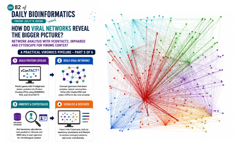
Mapping the Viral Universe: Network Analysis of Viral Communities with vConTACT2 and Cytoscape
🧬 𝐷𝑎𝑦 82 𝑜𝑓 𝐷𝑎𝑖𝑙𝑦 𝐵𝑖𝑜𝑖𝑛𝑓𝑜𝑟𝑚𝑎𝑡𝑖𝑐𝑠 𝑓𝑟𝑜𝑚 𝐽𝑜𝑗𝑦’𝑠 desk
Where we left off
Over the first four posts we identified viral genomes, clustered them into vOTUs, assigned taxonomy, measured abundance, identified auxiliary metabolic genes, predicted hosts, and determined lifestyle. Each of those analyses treats each vOTU independently — one row in a table.
But viruses do not exist independently. They share evolutionary history, exchange genes, and cluster into ecological guilds. Network analysis gives us a way to visualise all of those relationships at once, placing your environmental viruses in the context of the known viral universe and revealing structure that no table can show.
This post walks through the entire process from scratch — building a protein-sharing network with vConTACT2, importing it into Cytoscape, and decorating it with the taxonomy, abundance, host, and AMG data you have built up over the previous four days.
Part 1 — Why protein-sharing networks?
The limits of sequence identity clustering
In Day 1 we clustered viral contigs into vOTUs using 95% nucleotide identity over 85% alignment coverage. This is effective for grouping nearly identical sequences, but it tells us nothing about relationships between more divergent viruses.
Viral taxonomy itself has the same problem. Two phages can belong to the same family yet share only 30–40% average nucleotide identity. BLAST-based pairwise comparisons break down at these distances because viral proteins evolve so rapidly that nucleotide-level similarity disappears faster than functional or structural similarity.
Protein cluster networks: a better measure of relatedness
The solution used by vConTACT2 and other network-based tools is to work at the protein level rather than the nucleotide level. The logic is:
- Predict all proteins in all viral genomes
- Cluster those proteins into Protein Clusters (PCs) using pairwise DIAMOND alignments and MCL clustering — each PC represents a family of related proteins across your dataset
- Represent each viral genome as a set of PCs
- Connect two genomes with a weighted edge if they share one or more PCs — more shared PCs = stronger edge
- Apply a community detection algorithm (ClusterONE) to find Viral Clusters (VCs) — groups of genomes that are more connected to each other than to the rest of the network
This approach mirrors the way ICTV now classifies many viruses — shared gene content rather than sequence identity thresholds. It is far more sensitive to evolutionary relationships between divergent viruses, and it naturally places your environmental vOTUs in context alongside reference genomes.
What the network reveals
A vConTACT2 network typically shows:
- Dense clusters of closely related viruses (same family or genus)
- Singletons — your most novel viruses with no reference connections
- Bridge genomes — viruses that connect otherwise separate clusters, often representing recombination events or broad gene-sharing
- Your environmental vOTUs distributed across the reference landscape, some clustering tightly with known families and others floating in isolation
Every singleton is scientifically interesting. Every tight cluster with known references gives you high-confidence taxonomy. The bridges and overlaps tell you about viral evolution.
Part 2 — Installing vConTACT2
vConTACT2 is a Python tool with several external dependencies. Installation can be finicky — follow these steps carefully.
Important note: vConTACT2 is not always stable with the latest bioconda packages. If the conda install fails or produces errors, see the KBase alternative described in Part 7.
Dependencies
vConTACT2 requires:
- Python 3.9
- DIAMOND (for protein–protein alignment)
- BLAST (makeblastdb)
- MCL (Markov Cluster Algorithm)
- ClusterONE (JAR file, separate download)
- Prodigal (for ORF prediction — already installed from Day 2)
- Java (for ClusterONE)
Step 1 — Create the conda environment
module load anaconda3/2023.09-0

conda create \
  -p /your/tools/dir/vcontact2_env \
  -c conda-forge -c bioconda \
  --override-channels \
  python=3.9 vcontact2 prodigal diamond blast mcl \
  -y
The --override-channels flag forces conda to use only the specified channels, which reduces dependency conflicts that can otherwise cause vConTACT2 to install incorrectly.
Activate and verify:
conda activate /your/tools/dir/vcontact2_env
vcontact2 --help
Step 2 — Download ClusterONE
ClusterONE is a Java-based community detection algorithm required by vConTACT2. It is not available through conda and must be downloaded separately.
mkdir -p /your/tools/dir/clusterone

wget https://paccanarolab.org/static_content/clusterone/cluster_one-1.0.jar \
  -O /your/tools/dir/clusterone/cluster_one-1.0.jar

# Verify Java is available
java -version
If Java is not available on your system, load it as a module:
module load java/11.0.2   # adjust version to what your HPC provides
java -version
Step 3 — Verify the full setup
conda activate /your/tools/dir/vcontact2_env

# Check all dependencies are accessible
vcontact2 --help
diamond --version
mcl --version
java -jar /your/tools/dir/clusterone/cluster_one-1.0.jar --help
All four should produce output without errors.
Part 3 — Predicting proteins for vConTACT2
vConTACT2 works from predicted proteins, not nucleotide sequences. You need two files:
- A FASTA of all predicted protein sequences from your vOTUs (
vOTUs.faa) - A gene-to-genome mapping file that tells vConTACT2 which protein belongs to which viral genome
If you ran DRAM-v in Day 3, you already have genes.faa from the DRAM-v annotation output. You can use that directly, but you will need to standardise the headers. For simplicity, re-running Prodigal directly on vOTUs.fa is the cleanest approach.
Predict ORFs with Prodigal
module load prodigal/2.6.3

prodigal \
  -i vOTUs.fa \
  -a vOTUs.faa \
  -p meta \
  -f gff \
  -o vOTUs_prodigal.gff \
  -q
The -q flag suppresses verbose output. Check how many proteins were predicted:
grep -c '^>' vOTUs.faa
Create the gene-to-genome mapping file
vConTACT2 needs a CSV mapping each protein ID to its source genome. The vcontact2_gene2genome utility (installed with vConTACT2) generates this automatically from Prodigal output:
conda activate /your/tools/dir/vcontact2_env

vcontact2_gene2genome \
  -p vOTUs.faa \
  -o vOTUs_g2g.csv \
  -s Prodigal-FAA
Check the output:
head -5 vOTUs_g2g.csv
Expected format:
protein_id,contig_id,keywords
k141_1000054_1,k141_1000054,
k141_1000054_2,k141_1000054,
k141_1000076_1,k141_1000076,
Three columns: protein ID, genome (contig) ID, and keywords (usually empty for environmental sequences).
Part 4 — Running vConTACT2
Option A — vOTUs only (quick, no taxonomic context)
For a first run to understand your dataset’s internal structure:
conda activate /your/tools/dir/vcontact2_env

vcontact2 \
  --raw-proteins vOTUs.faa \
  --proteins-fp vOTUs_g2g.csv \
  --db None \
  --output-dir vcontact2_out \
  --pcs-mode MCL \
  --vcs-mode ClusterONE \
  --c1-bin /your/tools/dir/clusterone/cluster_one-1.0.jar \
  -t 16
Option B — vOTUs combined with INPHARED reference database (recommended)
INPHARED (INfrastructure for a PHAge REference Database) is a regularly updated collection of complete phage genomes with vConTACT2-formatted protein and gene-to-genome files. Including these references allows vConTACT2 to place your environmental vOTUs in the context of known phage diversity and dramatically improves taxonomic interpretation.
Download INPHARED:
mkdir -p /your/db/dir/inphared

# Download the most recent vConTACT2-ready files
# Check https://github.com/RyanCook94/inphared for current file names and dates
wget https://millardlab-inphared.s3.climb.ac.uk/1Sep2023_vConTACT2_proteins.faa.gz \
  -O /your/db/dir/inphared/inphared_proteins.faa.gz
wget https://millardlab-inphared.s3.climb.ac.uk/1Sep2023_data_excluding_refseq.tsv \
  -O /your/db/dir/inphared/inphared_metadata.tsv

gunzip /your/db/dir/inphared/inphared_proteins.faa.gz
You will also need the gene-to-genome file. For the most current files, visit github.com/RyanCook94/inphared and download the vConTACT2_g2g_table file corresponding to your protein download.
Combine with your vOTUs:
# Combine proteins
cat /your/db/dir/inphared/inphared_proteins.faa vOTUs.faa \
  > combined_proteins.faa

# Combine gene-to-genome files (skip header from vOTUs g2g)
cat /your/db/dir/inphared/inphared_g2g.csv \
    <(tail -n +2 vOTUs_g2g.csv) \
    > combined_g2g.csv

echo "Total proteins: $(grep -c '^>' combined_proteins.faa)"
echo "Total g2g rows: $(wc -l < combined_g2g.csv)"
Run vConTACT2 on the combined set:
conda activate /your/tools/dir/vcontact2_env

vcontact2 \
  --raw-proteins combined_proteins.faa \
  --proteins-fp combined_g2g.csv \
  --db None \
  --output-dir vcontact2_out_inphared \
  --pcs-mode MCL \
  --vcs-mode ClusterONE \
  --c1-bin /your/tools/dir/clusterone/cluster_one-1.0.jar \
  -t 16
This run will take significantly longer because of the reference proteins. On a 16-thread node, expect 2–8 hours depending on the size of your vOTU set.
Part 5 — Understanding vConTACT2 outputs
Key output files
vcontact2_out/
  genome_by_genome_overview.csv    ← main result: one row per genome
  c1.ntw                           ← weighted network edge list
  viral_cluster_overview.csv       ← one row per Viral Cluster
  PCs-proteins.csv                 ← protein cluster membership
  tax_predict_summary.csv          ← taxonomy prediction summary
  vConTACT2_log.txt                ← run log
genome_by_genome_overview.csv
This is the most important file for downstream analysis. It contains:
| Column | Description |
|---|---|
Genome | genome ID (your vOTU or INPHARED reference ID) |
VC | Viral Cluster assignment (e.g. VC_42) |
Status | Clustered, Singleton, Overlap, or Outlier |
VC Status | more detailed VC relationship |
Genus | predicted genus (if INPHARED references are in the same VC) |
Family | predicted family |
Order | predicted order |
Topology | network topology metric |
What the status values mean
| Status | Meaning | Ecological interpretation |
|---|---|---|
Clustered | Genome placed in a VC with at least one other genome | Known-ish virus — related to something in your dataset or the reference set |
Singleton | No shared PCs with any other genome | Highly novel; no detectable evolutionary relatives |
Overlap | Genome connects to more than one VC | May represent a mosaic virus bridging two lineages |
Outlier | Included in the network graph but not assigned to a VC | Has some connections but not enough for cluster assignment |
c1.ntw — the network edge list
This is a three-column file: genome_A, genome_B, weight. The weight reflects the number and quality of shared protein clusters. This file is what you import into Cytoscape to draw the network.
head -5 vcontact2_out/c1.ntw
k141_1000054  k141_1000076  12.4
k141_1000054  phage_reference_001  8.1
k141_1000076  phage_reference_002  15.7
Part 6 — Preparing the Cytoscape metadata file
Before importing into Cytoscape, prepare a node metadata table that combines all the ecology information you have built up in this series. This is what allows you to colour and size nodes by biology rather than just cluster membership.
The script 21_prepare_cytoscape_metadata.py in the repository handles this automatically. The key merging logic is:
import pandas as pd

# Load vConTACT2 genome overview
vc = pd.read_csv("vcontact2_out/genome_by_genome_overview.csv")
vc.rename(columns={"Genome": "vOTU"}, inplace=True)

# Load your master ecological table from Day 4
master = pd.read_csv("results/master_ecological_table.tsv", sep="\t")

# Join on vOTU ID
cyto_meta = vc.merge(master, on="vOTU", how="left")

# Add a column flagging your vOTUs vs reference genomes
cyto_meta["genome_type"] = cyto_meta["vOTU"].apply(
    lambda x: "environmental_vOTU"
    if x.startswith("k141_") or x.startswith("NODE_")
    else "reference_genome"
)

# Save as the Cytoscape node table
cyto_meta.to_csv("cytoscape_node_metadata.tsv", sep="\t", index=False)
print(f"Node metadata table: {cyto_meta.shape[0]} nodes × {cyto_meta.shape[1]} columns")
Part 7 — Visualising the network in Cytoscape
Cytoscape is a free, open-source network visualisation platform. Download it from cytoscape.org — it runs on Windows, macOS, and Linux.
Step 1 — Import the network
- Open Cytoscape
- Go to File → Import → Network from File
- Select
vcontact2_out/c1.ntw - In the import dialog:
- Column 1 → Source Node
- Column 2 → Target Node
- Column 3 → Edge Weight (set as a numeric attribute)
- Click OK
You should now see a hairball of nodes and edges. This is normal — we will apply a layout and style next.
Step 2 — Import the node metadata table
- Go to File → Import → Table from File
- Select
cytoscape_node_metadata.tsv - In the import dialog:
- Set Key Column for Network to match the node ID column (should be
vOTUorGenome) - Set Where to Import Table Data to
To a Network Collection
- Set Key Column for Network to match the node ID column (should be
- Click OK
All the metadata columns (family, host, lifestyle, abundance, AMG count, etc.) are now attached to the nodes and available for visual mapping.
Step 3 — Apply a layout
The default layout is usually unreadable. Apply a force-directed layout:
- Go to Layout → Prefuse Force Directed Layout → Edge Weight
This arranges nodes so that strongly connected genomes (many shared PCs) are pulled together, while weakly connected or unconnected genomes float apart. It takes 1–5 minutes for large networks.
Alternatively, try Layout → yFiles Organic Layout if you have the yFiles plugin installed — it handles large biological networks especially well.
Step 4 — Style nodes by taxonomy
Create a visual style that makes the taxonomy immediately visible:
- Open the Style panel (left sidebar)
- Click the + button to create a new style named
viromics_taxonomy
Node colour by viral family:
- Under Fill Color, click the dropdown and select Column: assigned_family
- Style: Discrete Mapping
- Assign colours to the top 10–15 families manually, or use a colour palette
- Use grey for “Unknown”
Node shape by genome type:
- Under Shape, select Column: genome_type
- Style: Discrete Mapping
- Environmental vOTUs → Circle
- Reference genomes → Square
Node size by mean relative abundance:
- Under Size, select Column: mean_relative_abundance
- Style: Continuous Mapping
- Map low abundance → small node (size 10), high abundance → large node (size 50)
- vOTUs with no abundance data → default size (15)
Node border colour by lifestyle:
- Under Border Paint, select Column: lifestyle
- Virulent → red border
- Temperate → blue border
- Unknown → grey border
Node label:
- Under Label, select Column: vOTU for your environmental nodes
- Optionally show only labels for specific nodes (highlight clusters of interest)
- Font size 6–8 works for dense networks
Step 5 — Style edges by weight
- Under Edge properties in the Style panel
- Width → Column: Edge Weight → Continuous Mapping
- Low weight → thin line (width 0.5), high weight → thick line (width 4)
- Transparency → set edges to ~60% opacity to reduce visual clutter
Step 6 — Highlight specific biology
Using Cytoscape’s Select tools, you can highlight subsets of nodes:
Select all vOTUs with AMGs:
- Go to Edit → Find or use the Filter panel
- Filter where
n_amgs > 0 - Change these nodes to a distinct colour (e.g. gold)
Select all temperate phages:
- Filter where
lifestyle == temperate - Add a distinct border or fill
Select a specific viral cluster:
- Filter where
VC == VC_42(replace with your cluster of interest) - Examine which reference genomes your environmental vOTUs cluster with
Step 7 — Export publication figures
- Go to File → Export → Network to Image
- Choose PDF for vector output (scalable for publication) or PNG at 300 DPI for presentations
- For a paper figure, export only the subnetwork of interest by selecting relevant nodes and using File → Export → Network to Image → Selected Nodes Only
Part 8 — Interpreting the network
Questions to ask of your network
How many of your vOTUs cluster with references? The fraction of Clustered vOTUs (with reference genomes in the same VC) is a measure of how well-characterised your viral community is. In a typical environmental dataset, 20–50% of vOTUs cluster with known phages. The rest are novel.
Which families dominate? Look at the large clusters in your network. If they are labelled with a known family (Drexlerviridae, Siphoviridae, etc.), your environment is relatively well-represented in reference databases. Large unlabelled clusters are priority targets for further study.
Are AMG-carrying vOTUs clustered or singleton? If your most ecologically interesting vOTUs (those with AMGs for photosynthesis or sulfur cycling) are singletons, they represent novel viral lineages performing known metabolic functions — a finding worth highlighting. If they cluster with known phages, you have reference context for understanding them.
Where do temperate phages sit in the network? In many environmental datasets, temperate phages form distinct clusters from virulent ones. If you have added lifestyle as a node attribute, look at whether the VC clusters separate by lifestyle or whether lytic and lysogenic phages intermix within clusters.
Bridge genomes — mosaic evolution in action? Any Overlap nodes connecting multiple clusters are potential mosaic genomes — viruses that have exchanged genomic modules with multiple lineages. These are rare but scientifically fascinating and often flag horizontal gene transfer events.
Part 9 — KBase: a web alternative for vConTACT2
If you have trouble installing vConTACT2 locally, or if you want to try the analysis without an HPC account, KBase offers a free browser-based platform where you can run vConTACT2 as a GUI app.
What is KBase?
KBase (kbase.us) is a US Department of Energy platform for comparative genomics and metagenomics. It provides a Jupyter-like Narrative interface where you can upload data, run analysis apps, and share results — all in a web browser, no installation required.
Running vConTACT2 on KBase
-
Create a free account at kbase.us
-
Create a new Narrative (think of it as a project workspace)
- Upload your data:
- In the Data panel (left sidebar), click Import
- Upload your
vOTUs.faas a FASTA file
- Find the vConTACT2 app:
- In the Apps panel, search for
vConTACT2 - Click the app to add it to your Narrative
- In the Apps panel, search for
- Configure the app:
- Input genome set: select your uploaded
vOTUs.fa - Reference database: select
INPHARED(available as a preloaded option) - PCs mode:
MCL - VCs mode:
ClusterONE - Leave other settings at defaults for a standard run
- Input genome set: select your uploaded
-
Run the app — click the play button and wait. KBase allocates compute resources automatically. Runtime is similar to a local HPC run.
- Download outputs:
- The app produces
genome_by_genome_overview.csvandc1.ntwas downloadable files - Download these and proceed with Cytoscape visualisation as described in Part 7
- The app produces
KBase limitations: The free tier has storage and compute limits. For very large datasets (>5000 vOTUs + INPHARED references) a local HPC run is more practical. KBase is ideal for the toy dataset, for learning, and for datasets up to a few thousand sequences.
Part 10 — Other tools for viral network analysis
vcluster / vcluster2
A streamlined reimplementation of the vConTACT2 concept designed for better scalability and easier installation. Worth trying if vConTACT2’s dependency chain causes problems.
PhaGCN2
GitHub: github.com/KennthShang/PhaGCN2
Uses graph convolutional networks rather than protein-cluster community detection. Assigns taxonomy to phages using a GCN trained on known phage genomes. Particularly good for novel phages where the protein-sharing signal to reference databases is weak. Outputs taxonomy assignments that can be used as node colours in Cytoscape even when vConTACT2 returns many unknowns.
VICTOR
A genome-based phylogeny tool that produces trees (rather than networks) based on intergenomic distances. Useful when you want a phylogenetic tree for a specific viral cluster rather than a whole-dataset network.
VIRIDIC
Calculates intergenomic similarity between phage genomes and classifies them according to ICTV species and genus thresholds. A complement to vConTACT2 rather than a replacement — VIRIDIC is better for precise species-level demarcation within a family, while vConTACT2 gives a broader community-level view.
anvi’o pan-genomics module
If you are already using anvi’o (a popular metagenomics platform), its pan-genomics module can produce protein-sharing networks for viral genomes and visualise them in anvi’o’s interactive interface. The visual output is different from Cytoscape but is often easier to annotate interactively.
Part 11 — What you have at the end of Day 5
| File | Contents |
|---|---|
vOTUs.faa | Prodigal-predicted proteins from all vOTUs |
vOTUs_g2g.csv | Gene-to-genome mapping file |
vcontact2_out/genome_by_genome_overview.csv | VC assignments and status for all genomes |
vcontact2_out/c1.ntw | Weighted network edge list for Cytoscape |
cytoscape_node_metadata.tsv | All ecology metadata joined to genome IDs |
Cytoscape session file (.cys) | Your annotated, styled network |
| Exported network figure (PDF/PNG) | Publication-ready network visualisation |
In the final post — Day 6 — we add the last layer of information: activity. We will map metatranscriptomic reads to your viral genomes and AMG-carrying contigs to identify which viruses are actively transcribing in your samples, which AMGs are being expressed during active infection, and how to interpret active viral communities in the context of everything we have built over this series.
Companion repository: metagenome-to-viromics Scripts, and install guides for every step in this series live here. Day 2 materials are in
day5/. Today’s image is a simplified toy visualization created for demonstration purposes only.