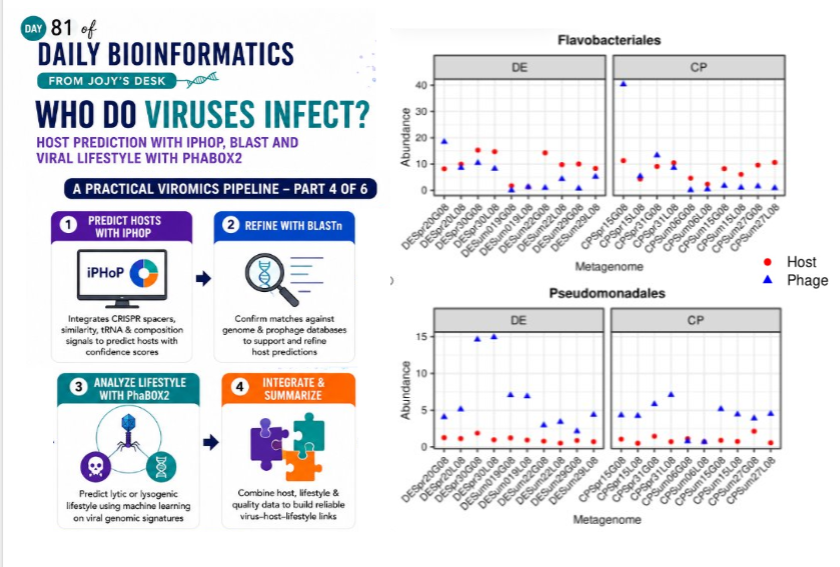
Who Do Viruses Infect? Host Prediction with iPHoP, BLAST, and Viral Lifestyle with PhaBOX2
Where we left off
🧬 𝐷𝑎𝑦 81 𝑜𝑓 𝐷𝑎𝑖𝑙𝑦 𝐵𝑖𝑜𝑖𝑛𝑓𝑜𝑟𝑚𝑎𝑡𝑖𝑐𝑠 𝑓𝑟𝑜𝑚 𝐽𝑜𝑗𝑦’𝑠 desk
Over the first three posts we assembled a picture of the viral community in our environmental samples: we identified viral genomes, clustered them into vOTUs, assessed their quality, assigned taxonomy, measured abundance, and identified the auxiliary metabolic genes they carry.
But there is a gap at the centre of everything. When a phage is listed as belonging to Drexlerviridae with an AMG for sulfur metabolism — who exactly is it infecting? And when it infects, does it kill the host immediately or slip quietly into the chromosome and wait?
Those two questions — who is the host? and what is the lifestyle? — are the subject of this post.
Part 1 — Why host prediction matters
Virus–host interactions drive nearly every ecological process that viruses are involved in. Lysis releases nutrients. Lysogeny modifies host gene expression. AMGs only make biological sense once you know which host metabolic pathway the phage is supplementing during infection. And host range data is essential for building interaction networks — the ecological wiring diagrams that connect viral diversity to microbial community dynamics.
The problem is that most environmental viruses have never been cultured alongside their hosts. We cannot grow the virus and the host together in a flask and observe infection directly. Instead we have to infer the host from genomic signals in the assembled sequences.
What signals connect a virus to its host?
Several types of molecular evidence can link a viral genome to a microbial host:
CRISPR spacer matches. CRISPR-Cas systems are adaptive immune systems found in many bacteria and archaea. When a cell survives a viral infection, it can incorporate a short segment of viral sequence (a spacer) into its CRISPR array. If we find a CRISPR spacer in a microbial genome that matches a sequence in our viral contig, that is direct molecular evidence of a past infection event — one of the strongest possible signals.
Sequence similarity (BLASTn). Prophages — viral genomes integrated into host chromosomes — leave traces in bacterial genome sequences. If our viral contig shares significant nucleotide similarity with a prophage region in a reference bacterial genome, the host of that reference genome is a plausible host for our virus.
tRNA matches. Some phages insert their genomes next to tRNA genes during integration. Finding a tRNA sequence at the junction of a viral contig and an adjacent contig can point to a host lineage.
k-mer composition similarity. Viral genomes and their hosts share subtle nucleotide composition signatures (codon usage, GC content patterns) that evolve together over long evolutionary timescales. These signals are weaker than CRISPR or similarity matches but can be informative when nothing else is available.
Machine learning integration. Modern tools like iPHoP combine all of these signals using an ensemble of models, assigning a confidence score to each prediction.
Part 2 — iPHoP: integrated host prediction
iPHoP (integrated Phage Host Prediction) is currently the most comprehensive tool for environmental virus host prediction. It integrates predictions from multiple methods — CRISPR spacer matching, sequence similarity, tRNA-based matching, and composition-based models — and reports a confidence score for each prediction.
Publication: Roux et al. (2023) PLOS Biology doi:10.1371/journal.pbio.3002083
GitHub: github.com/sib-swiss/iPHoP
Installing iPHoP
module load anaconda3/2023.09-0

conda create \
  -p /your/tools/dir/iphop_env \
  -c conda-forge -c bioconda \
  iphop \
  -y

conda activate /your/tools/dir/iphop_env
iphop -h
Downloading the iPHoP database
The iPHoP database contains microbial reference genomes, precomputed CRISPR spacer arrays, prophage regions, and model parameters. It is large (~80–100 GB after decompression).
mkdir -p /your/db/dir/iphop_db

conda activate /your/tools/dir/iphop_env

iphop download \
  --db_dir /your/db/dir/iphop_db \
  --full_offline
The --full_offline flag downloads everything needed for offline use. This can take several hours. On an HPC system with a slow external connection, plan to submit a download job overnight.
You can also check for the latest available database version before downloading:
iphop download --list
Running iPHoP
conda activate /your/tools/dir/iphop_env

iphop predict \
  --fa_file vOTUs.fa \
  --db_dir /your/db/dir/iphop_db \
  --out_dir iphop_output \
  --num_threads 16
Key parameters:
| Parameter | Meaning |
|---|---|
--fa_file | your vOTUs FASTA |
--db_dir | path to the downloaded iPHoP database |
--out_dir | output directory |
--num_threads | threads to use |
--min_score | minimum confidence score to report (default 90) |
iPHoP output files
iphop_output/
  Host_prediction_to_genus_m90.csv     ← main result file
  Host_prediction_to_genome_m90.csv    ← genome-level predictions
  Detailed_output_by_tool/             ← per-method breakdown
    CRISPR_based_predictions.csv
    Blast_based_predictions.csv
    RaFAH_based_predictions.csv
    ...
The main file is Host_prediction_to_genus_m90.csv. The m90 suffix indicates that only predictions with a confidence score ≥ 90 are included.
Key columns in the output:
| Column | Description |
|---|---|
Virus | viral genome (vOTU) ID |
AAI to closest RaFAH hit | average amino acid identity to closest reference |
Host genus | predicted host at genus level |
Host lineage | full predicted host taxonomy |
Confidence score | overall prediction confidence (0–100) |
Method(s) | which method(s) supported this prediction |
Filtering by confidence
A confidence score ≥ 90 is the standard threshold for reporting host predictions with high confidence. iPHoP uses this as the default. For exploratory analysis you may lower it to 75 to recover more predictions at reduced confidence:
iphop predict \
  --fa_file vOTUs.fa \
  --db_dir /your/db/dir/iphop_db \
  --out_dir iphop_output_m75 \
  --num_threads 16 \
  --min_score 75
For publication-quality results, use the 90 threshold unless you have a specific reason to lower it.
What iPHoP host predictions look like
In a typical environmental metagenome analysis, iPHoP will assign host predictions to 30–70% of vOTUs at the 90% confidence threshold. The remainder have no prediction — either because no closely related viruses are in the database, or because the viral genome is too short or too novel for any method to match.
Predicted hosts cluster around the dominant bacteria in your system. In a marine metagenome, you will see many predictions to Pelagibacter, Prochlorococcus, Alteromonas, and Roseobacter lineages. In a soil or estuarine dataset, predictions shift toward Proteobacteria, Actinobacteria, Firmicutes, and Bacteroidetes.
Part 3 — BLAST-based host prediction
iPHoP integrates BLAST internally, but running a standalone BLASTn search against a curated microbial genome database gives you full control and transparency over the matching process. This is particularly useful for:
- Confirming iPHoP predictions with an independent line of evidence
- Finding host matches in custom databases not included in iPHoP
- Investigating specific high-interest vOTUs in detail
The logic: prophage similarity
Most bacterial genomes contain prophages — remnants of past viral infections that integrated and were retained. If your environmental viral contig shares strong nucleotide similarity (typically >70% identity over >50% of the contig length) with a prophage region in a reference genome, that reference bacterium is a plausible host.
Building the reference database
For a general-purpose host prediction BLAST database, use a curated set of bacterial and archaeal reference genomes. The NCBI RefSeq representative genome set is a good starting point:
module load ncbi-blast+/2.17.0

# Create database directory
mkdir -p /your/db/dir/host_blast_db

# Option A: use a pre-downloaded genome set (recommended for HPC)
# Concatenate all reference genome FASTA files
cat /path/to/reference_genomes/*.fna > all_host_genomes.fna

# Build BLAST nucleotide database
makeblastdb \
  -in all_host_genomes.fna \
  -dbtype nucl \
  -out /your/db/dir/host_blast_db/host_genomes \
  -title "Host_genomes_RefSeq" \
  -parse_seqids
If you have MAGs (metagenome-assembled genomes) from the same samples, include them — they are likely to contain prophages from the viruses you are studying and will give the most relevant matches.
Running BLASTn
module load ncbi-blast+/2.17.0

blastn \
  -query vOTUs.fa \
  -db /your/db/dir/host_blast_db/host_genomes \
  -evalue 1e-5 \
  -outfmt "6 qseqid sseqid pident length qlen slen evalue bitscore staxids sscinames" \
  -num_threads 16 \
  -max_target_seqs 5 \
  -perc_identity 70 \
  -out blastn_vs_host_genomes.txt
Additional filter flags explained:
| Flag | Value | Meaning |
|---|---|---|
-perc_identity | 70 | require at least 70% nucleotide identity |
-max_target_seqs | 5 | return at most 5 best hits per query |
-evalue | 1e-5 | maximum E-value to report |
Post-processing BLAST hits
For a hit to suggest a host relationship, a common threshold is:
- ≥ 70% nucleotide identity
- ≥ 50% alignment coverage of the viral contig
# Filter BLAST hits: ≥70% identity, alignment covers ≥50% of query
awk -F'\t' 'NR>1 && $3>=70 && ($4/$5)>=0.5 {print}' \
  blastn_vs_host_genomes.txt \
  > blastn_host_filtered.txt

echo "Hits passing filter: $(wc -l < blastn_host_filtered.txt)"
The Python script 16_blast_host_prediction.py in the repository handles this filtering, extracts the best hit per vOTU, and produces a clean host prediction table ready for joining with your taxonomy and AMG data.
Part 4 — CRISPR spacer matching (standalone approach)
iPHoP performs CRISPR matching internally, but if you want to run it independently — for example, using your own MAG-derived CRISPR arrays — the steps are straightforward.
Predicting CRISPR spacers in MAGs
CRISPRDetect or MinCED can identify CRISPR arrays in your microbial genomes:
# Using MinCED (fast, conda installable)
conda activate /your/tools/dir/minced_env

for MAG in /path/to/mags/*.fna; do
  STEM=$(basename "$MAG" .fna)
  minced \
    -spacers \
    "$MAG" \
    mags_crispr/${STEM}.crispr \
    mags_crispr/${STEM}_spacers.fa
done

# Combine all spacers into one file
cat mags_crispr/*_spacers.fa > all_crispr_spacers.fa
wc -l all_crispr_spacers.fa
Matching spacers to viral contigs
# Build a BLAST database from viral contigs
makeblastdb \
  -in vOTUs.fa \
  -dbtype nucl \
  -out crispr_blast_db/vOTUs

# BLAST spacers against viral contigs
blastn \
  -query all_crispr_spacers.fa \
  -db crispr_blast_db/vOTUs \
  -task blastn-short \
  -perc_identity 95 \
  -evalue 1 \
  -outfmt "6 qseqid sseqid pident length mismatch gapopen evalue bitscore" \
  -num_threads 16 \
  -out crispr_spacer_hits.txt
Why
blastn-shortandperc_identity 95? CRISPR spacers are very short (~30–40 bp). Standard BLASTn settings are optimised for longer queries and will miss short matches.blastn-shortadjusts the word size and scoring for short queries. The 95% identity threshold is standard for CRISPR matching — spacers diverge rapidly, so only near-perfect matches are considered meaningful.
A spacer hit means the MAG from which that spacer came has previously encountered a virus matching that vOTU. The MAG organism is therefore a confirmed (or historically confirmed) host.
Part 5 — Merging host predictions
You now potentially have host predictions from three sources:
- iPHoP (integrated, confidence-scored)
- BLASTn against reference genomes
- CRISPR spacer matching against MAGs
The Python script 16_blast_host_prediction.py in the repository merges these into a single host prediction table with source tracking and a simple priority scheme:
CRISPR match (≥95% identity)   →  highest confidence
iPHoP (≥90 confidence score)   →  high confidence
BLASTn (≥70% id, ≥50% coverage)→  moderate confidence
When multiple sources agree on the same host lineage, confidence increases further. When they disagree, all predictions are retained with their source labelled so you can decide how to interpret them.
Part 6 — Interpreting host predictions ecologically
Linking hosts to AMGs
Once you have host predictions, you can finally give ecological meaning to the AMGs you found in Day 3. If a vOTU is predicted to infect a sulfate-reducing bacterium and carries dsrA — the key gene in dissimilatory sulfate reduction — that is a coherent biological story: the virus is manipulating its host’s core energy metabolism during infection.
Cross-reference your merged AMG-taxonomy table with host predictions:
import pandas as pd

amg  = pd.read_csv("results/amg_taxonomy_vitap_merged.tsv", sep="\t")
host = pd.read_csv("iphop_output/Host_prediction_to_genus_m90.csv")
host.rename(columns={"Virus": "vOTU"}, inplace=True)

merged = amg.merge(
    host[["vOTU", "Host genus", "Host lineage", "Confidence score"]],
    on="vOTU", how="left"
)
merged.to_csv("results/amg_host_merged.tsv", sep="\t", index=False)
print(merged[["vOTU", "kegg_hit", "best_family", "Host genus"]].head(20).to_string())
Host range patterns
Do the viruses in your dataset show broad or narrow host range? If a single vOTU gets CRISPR spacer matches from multiple distantly related bacterial genera, it may be a generalist phage. If all predictions point to a single host genus, it is likely a specialist. This matters for modelling — specialist phages drive boom-bust dynamics in specific host populations, while generalists can affect community diversity more broadly.
Connecting to ecosystem function
In nutrient cycling contexts, the most ecologically meaningful result is identifying which functional guilds are being infected. For example:
- Viruses infecting nitrifiers (Nitrosomonas, Nitrospira) can suppress nitrification rates
- Viruses infecting methanotrophs can affect methane oxidation
- Viruses infecting primary producers (Prochlorococcus, diatoms) affect carbon export
Part 7 — Viral lifestyle prediction with PhaBOX2
Host prediction tells you who the virus infects. Lifestyle prediction tells you how — does the virus immediately kill the host (lytic/virulent), or does it integrate into the host genome and remain dormant (lysogenic/temperate)?
This distinction has major ecological consequences.
Lytic vs lysogenic: why it matters
Virulent (lytic) phages infect a cell, replicate rapidly, and lyse it — releasing hundreds of new phage particles and the cell’s nutrients back into the environment. This drives the viral shunt of nutrient cycling. High lytic activity means rapid microbial turnover and carbon flux.
Temperate (lysogenic) phages can integrate their DNA into the host chromosome as a prophage. The virus then replicates silently with the host cell across many generations. The host is not immediately killed. The prophage can, however, be induced — by UV light, DNA damage, or other stressors — to excise and enter the lytic cycle. Temperate phages can also carry and transfer genes between hosts through lysogenic conversion.
The balance between lytic and lysogenic lifestyles in an environment is not fixed. In nutrient-rich conditions with fast-growing bacteria, lytic infections tend to dominate (the “Piggyback-the-Winner” hypothesis in reverse). In nutrient-poor, stressed conditions, lysogeny tends to increase. Understanding which lifestyle dominates in your samples connects viral ecology to the broader environmental context.
PhaBOX2
PhaBOX2 is a deep-learning-based tool that predicts viral lifestyle (and other properties) from genome sequence alone. It uses protein language model-derived embeddings and transformer-based neural networks to classify viruses as virulent or temperate.
GitHub: github.com/KennthShang/PhaBOX
Publication: Shang et al. (2024)
Installing PhaBOX2
module load anaconda3/2023.09-0

conda create -n phabox2_env python=3.9 -y
conda activate phabox2_env

pip install phabox2

phabox2 -h
Downloading the PhaBOX2 database
mkdir -p /your/db/dir/phabox2_db

conda activate phabox2_env

phabox2 download-database \
  --db_dir /your/db/dir/phabox2_db
The database contains pre-trained deep learning model weights. It is ~5–10 GB and downloads in 15–30 minutes.
Running lifestyle prediction
conda activate phabox2_env

phabox2 predict \
  -i vOTUs.fa \
  -o phabox2_output \
  -d /your/db/dir/phabox2_db \
  -t 16
PhaBOX2 output
phabox2_output/
  lifestyle_prediction.tsv    ← main result
  taxonomy_prediction.tsv     ← PhaBOX2 taxonomy (bonus output)
  host_prediction.tsv         ← basic host prediction (bonus output)
lifestyle_prediction.tsv columns:
| Column | Meaning |
|---|---|
virus_id | vOTU ID |
lifestyle | virulent or temperate |
confidence | prediction confidence score (0–1) |
Interpreting PhaBOX2 results
| Prediction | Biological meaning | Ecological implication |
|---|---|---|
virulent | strictly lytic phage | drives host turnover, nutrient cycling, viral shunt |
temperate | capable of lysogeny | integrates into host, can be induced, enables gene transfer |
Confidence thresholds to use:
-
≥ 0.9— high confidence, report as confident prediction -
0.7–0.9— moderate confidence, report with caveat -
< 0.7— low confidence, treat as uncertain
Validating temperate predictions
For vOTUs predicted as temperate with high confidence, check whether DRAM-v identified any of the hallmark lysogeny genes:
| Gene | Function |
|---|---|
| Integrase / tyrosine recombinase | mediates phage integration into host chromosome |
| Serine recombinase | alternative integration mechanism |
| CI repressor / lysogeny repressor | suppresses lytic genes during lysogeny |
| Excisionase (Xis) | mediates prophage excision |
| Recombinase | used in some integration systems |
# Quick search for integrase annotations in DRAM-v output
grep -i "integrase\|recombinase\|repressor\|excisionase" \
  dramv_annotate/annotations.tsv | \
  cut -f1,2,8,9 | head -20
If PhaBOX2 calls a vOTU as temperate AND DRAM-v finds an integrase in the same contig, confidence in the temperate call is very high.
Part 8 — Combining host prediction and lifestyle: ecological interpretation
When you combine host identity (from iPHoP) with lifestyle (from PhaBOX2), you can build a rich ecological picture for each vOTU. Some examples of what this combination reveals:
Temperate phage infecting a dominant bacterium This virus is likely integrated into many cells of that host in your environment. It is not causing visible mortality but may be transferring genes, modifying host surface proteins (lysogenic conversion), or sitting silently waiting for an induction trigger. If the host is abundant, this virus represents a substantial reservoir of viral DNA moving with the host population.
Virulent phage infecting a keystone species A lytic phage that kills a numerically or functionally important microorganism can reshape the whole community. If the host is a nitrogen fixer, a primary producer, or a major decomposer, viral lysis can interrupt a key ecological function seasonally or episodically.
Temperate phage with AMGs This combination is particularly interesting. Temperate phages that carry AMGs do not just express those genes during lytic infection — they may also express them during lysogeny, constitutively modifying the host’s metabolism. Phages carrying photosynthesis or nutrient acquisition genes that are also temperate may be providing persistent metabolic benefits to the host lineage.
Part 9 — Merging everything: the master ecological table
At the end of Day 4 you have all the major pieces:
- Taxonomy (Day 2): what viral family each vOTU belongs to
- Abundance (Day 2): how many reads map to each vOTU in each sample
- AMGs (Day 3): what metabolic functions each vOTU carries
- Host prediction (Day 4): what microbial genus each vOTU infects
- Lifestyle (Day 4): whether each vOTU is virulent or temperate
Joining all of these on vOTU ID gives you a master ecological table that is the basis for all downstream ecological analysis, network visualisation, and statistical testing.
The script 17_build_master_table.py in the repository performs this join, fills missing values sensibly, and produces a final summary.
import pandas as pd

# Load all tables
tax    = pd.read_csv("results/master_taxonomy.tsv", sep="\t")
abund  = pd.read_csv("results/coverm_abundance_filtered.tsv", sep="\t", index_col=0)
amg    = pd.read_csv("results/amg_taxonomy_vitap_merged.tsv", sep="\t")
host   = pd.read_csv("iphop_output/Host_prediction_to_genus_m90.csv")
life   = pd.read_csv("phabox2_output/lifestyle_prediction.tsv", sep="\t")

host.rename(columns={"Virus": "vOTU"}, inplace=True)
life.rename(columns={"virus_id": "vOTU"}, inplace=True)

# Build master per-vOTU table
master = tax.merge(host[["vOTU", "Host genus", "Host lineage", "Confidence score"]],
                   on="vOTU", how="left")
master = master.merge(life[["vOTU", "lifestyle", "confidence"]],
                      on="vOTU", how="left")

# Add mean abundance
ra_cols = [c for c in abund.columns if "Relative Abundance" in c]
abund_mean = abund[ra_cols].mean(axis=1).rename("mean_relative_abundance")
abund_mean.index.name = "vOTU"
master = master.merge(abund_mean.reset_index(), on="vOTU", how="left")

# Add AMG count per vOTU
if "vOTU" in amg.columns:
    amg_counts = amg.groupby("vOTU").size().rename("n_amgs").reset_index()
    master = master.merge(amg_counts, on="vOTU", how="left")
    master["n_amgs"] = master["n_amgs"].fillna(0).astype(int)

master.to_csv("results/master_ecological_table.tsv", sep="\t", index=False)
print(f"Master table: {master.shape[0]} vOTUs × {master.shape[1]} columns")
print(master[["vOTU", "assigned_family", "Host genus", "lifestyle", "n_amgs",
              "mean_relative_abundance"]].head(10).to_string())
Part 10 — A note on other tools for host prediction and lifestyle
RaFAH
GitHub: github.com/felipehcoutinho/RaFAH
Random Forest Assignment of Hosts (RaFAH) predicts virus–host relationships using a random forest classifier trained on protein-level features. It is one of the methods integrated inside iPHoP, but can also be run standalone if you want direct access to its predictions or need to run on a custom host reference set.
CHERRY
GitHub: github.com/KennthShang/CHERRY
CHERRY predicts phage hosts using a knowledge graph-based approach that combines protein similarity and co-occurrence patterns. It performs well on novel phages with limited database similarity and is worth considering when iPHoP returns few predictions.
DeepHost
A deep learning approach for phage host prediction using convolutional neural networks on sequence composition features. Useful as a sanity check for predictions from other tools.
VIBRANT lifestyle prediction
VIBRANT (introduced in Day 3 as an alternative to DRAM-v) also includes lifestyle prediction as part of its pipeline, classifying phages as lytic or lysogenic. If you used VIBRANT for AMG annotation, its lifestyle calls are available without running an additional tool. However, PhaBOX2 is generally considered more accurate for this specific task.
CheckV provirus detection (revisited)
In Day 1 we used CheckV primarily for quality assessment. Its proviruses.fna output is also directly relevant to lifestyle — sequences placed in proviruses.fna are viral regions embedded in host scaffolds, which by definition represent temperate phages in their integrated (lysogenic) state. If your metagenome assembly produced long scaffolds with both host and viral regions, CheckV’s provirus calls are direct evidence of lysogeny.
Part 11 — What you have at the end of Day 4
| File | Contents |
|---|---|
iphop_output/Host_prediction_to_genus_m90.csv | iPHoP host predictions (genus level, ≥90 confidence) |
blastn_host_filtered.txt | BLASTn host predictions (filtered) |
crispr_spacer_hits.txt | CRISPR spacer matches (if MAGs available) |
results/host_predictions_combined.tsv | merged host predictions from all methods |
phabox2_output/lifestyle_prediction.tsv | PhaBOX2 lifestyle calls |
results/amg_host_merged.tsv | AMGs joined with host predictions |
results/master_ecological_table.tsv | all data joined per vOTU |
In the next post — the final one in this series — we shift from DNA to RNA. We will use metatranscriptomic data to identify which viral genomes are actively transcribed in your samples, which AMGs are being expressed during infection, and how to connect transcriptional activity to the ecological roles we have been building toward throughout this series.
Companion repository: metagenome-to-viromics Scripts, and install guides for every step in this series live here. Day 2 materials are in
day4/.