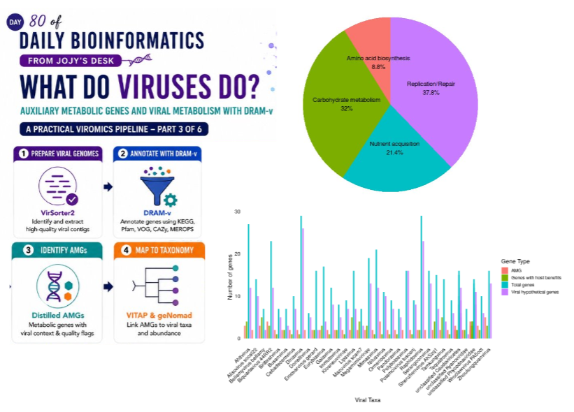
What Do Viruses Do? Auxiliary Metabolic Genes and Viral Metabolism with DRAM-v
Where we left off
🧬 𝐷𝑎𝑦 80 𝑜𝑓 𝐷𝑎𝑖𝑙𝑦 𝐵𝑖𝑜𝑖𝑛𝑓𝑜𝑟𝑚𝑎𝑡𝑖𝑐𝑠 𝑓𝑟𝑜𝑚 𝐽𝑜𝑗𝑦’𝑠 desk
In the previous two posts we went from a raw metagenomic assembly to a set of quality-filtered viral OTUs (vOTUs.fa), assigned them taxonomy using geNomad and BLAST, and estimated their abundance across samples with Bowtie2 and CoverM.
We now know who the viruses are and how many of them are present. But there is a third question that is arguably the most ecologically exciting: what are they doing?
Part 1 — Viruses as metabolic engineers
The traditional view of a bacteriophage is simple: it injects DNA, hijacks the host’s machinery, makes copies of itself, and bursts the cell open. Kill, release, repeat. But this picture is incomplete in a way that matters enormously for how we understand ecosystems.
A large and growing fraction of environmental viral genomes carry auxiliary metabolic genes — abbreviated AMGs. These are host-derived genes that viruses have captured and integrated into their own genomes. During infection, the virus expresses these genes to redirect or supplement host metabolism in ways that benefit viral replication.
The critical word is auxiliary. These genes do not help the virus replicate directly in the way that capsid or tail fibre genes do. Instead they tweak the metabolic environment the virus finds itself in — boosting energy production, bypassing metabolic bottlenecks, or diverting cellular resources toward nucleotide synthesis.
Examples from the real world
Photosystem II genes in cyanophages. Marine cyanobacteria of the genus Prochlorococcus and Synechococcus are responsible for a significant fraction of global ocean primary productivity. Cyanophages that infect them frequently carry psbA — the gene encoding the D1 protein of Photosystem II. During infection the host’s D1 protein is degraded by high-light stress, but the phage-encoded copy keeps photosynthesis running, sustaining the ATP and NADPH supply the phage needs to replicate. The phage is essentially keeping the lights on in a cell it is about to destroy.
Phosphorus acquisition genes. In phosphorus-limited marine environments, phages carry phoH and pstS genes involved in phosphate uptake. By expressing these during infection, the virus maximises phosphorus availability for nucleotide synthesis.
Sulfur metabolism genes. In deep-sea and estuarine environments, viruses carry genes from the dissimilatory sulfite reductase pathway (dsrA, dsrB, dsrC) and the sulfate adenylyltransferase pathway (sat, aprA, aprB). These AMGs can influence the sulfur cycle at the community level.
Carbon metabolism genes. Genes from glycolysis (pykA, zwf), the TCA cycle (sucA, sdhA), and fatty acid biosynthesis have all been documented as AMGs. In organic-rich environments, these can enhance energy availability during the burst of viral replication.
The ecosystem-level consequence
When a phage carrying an AMG infects a cell, it does not just consume that cell — it temporarily reprogrammes it. A cell infected by a psbA-carrying phage continues fixing carbon (for the phage’s benefit) until lysis. Multiply this across billions of infections per millilitre of seawater and you have a detectable biogeochemical signal. AMGs are one mechanism by which viral activity is coupled to elemental cycling, and understanding them is essential for building accurate models of microbial ecosystem function.
Part 2 — How AMGs are identified: the DRAM-v approach
The challenge with identifying AMGs is distinguishing them from other viral genes. A viral genome contains three broad categories of genes:
- Viral structural and replication genes — capsid proteins, tail fibres, DNA polymerases, terminases. These are the core viral machinery.
- Auxiliary metabolic genes — metabolic genes of clearly host origin that are expressed during infection.
- Unknown genes — the majority of genes in any environmental viral genome have no known function.
DRAM-v (Distilled and Refined Annotation of Metabolism — viral) addresses this by:
- Annotating every predicted gene in a viral contig against multiple databases simultaneously: KEGG, Pfam, VOG (Viral Orthologous Groups), CAZy (carbohydrate-active enzymes), and MEROPS (peptidases).
- Using VOG annotations to identify genes with viral hallmarks.
- Flagging genes that have metabolic annotations (from KEGG/Pfam) but no or weak viral hallmark support — these are candidate AMGs.
- Adding quality flags based on gene position (near contig end), proximity to transposons, and whether the surrounding gene neighbourhood looks viral.
- Distilling the annotation into a summary table of AMG calls with confidence flags.
The combination of multiple databases and the distillation step is what makes DRAM-v powerful. It does not just ask “is this gene metabolic?” — it asks “is this gene metabolic AND embedded in a viral genomic context AND not next to a transposon AND not at a contig edge that might represent host contamination?”
Part 3 — Preparing inputs: VirSorter2 in DRAM-v mode
DRAM-v requires a specific input format produced by VirSorter2. You need to re-run VirSorter2 on your final vOTUs.fa with the --prep-for-dramv flag. This produces two files that DRAM-v needs:
-
final-viral-combined-for-dramv.fa— the viral sequences with DRAM-v-compatible headers -
viral-affi-contigs-for-dramv.tab— a gene affiliation table that tells DRAM-v which genes have viral hallmark support
This is a separate VirSorter2 run from the one in Day 1. That run was to identify viral contigs from the raw assembly. This run is specifically to prepare the annotation input for DRAM-v, so it is run on the already-filtered vOTUs.fa.
Re-running VirSorter2 with –prep-for-dramv
conda activate /path/to/virsorter2_env

virsorter run \
  -i vOTUs.fa \
  -w virsorter2_dramv_prep \
  --db-dir /path/to/virsorter2_db \
  --min-length 1000 \
  --include-groups "dsDNAphage,ssDNA,RNA,NCLDV,lavidaviridae" \
  --prep-for-dramv \
  -j 16 \
  all
The key difference from the Day 1 run is --prep-for-dramv. The minimum length is also set to 1000 bp here (lower than the 1500 bp used for initial identification) because we are already working with quality-filtered vOTUs and want to retain as many as possible for annotation.
This will produce:
virsorter2_dramv_prep/for-dramv/
  final-viral-combined-for-dramv.fa
  viral-affi-contigs-for-dramv.tab
Part 4 — Installing DRAM-v
DRAM (Distilled and Refined Annotation of Metabolism) is a comprehensive annotation tool with a large database set. The installation is somewhat involved — plan for several hours for database download.
Environment setup
module load anaconda3/2023.09-0

conda create \
  -p /your/tools/dir/DRAM_env \
  -c conda-forge -c bioconda \
  dram \
  -y

conda activate /your/tools/dir/DRAM_env
DRAM-v.py --help
Database setup
DRAM requires several large databases. The DRAM-setup.py command downloads and configures all of them:
conda activate /your/tools/dir/DRAM_env

mkdir -p /your/db/dir/DRAM_db

DRAM-setup.py prepare_databases \
  --output_dir /your/db/dir/DRAM_db \
  --threads 16 \
  --skip_uniref       # skip UniRef90 to save time/space (~100 GB)
About
--skip_uniref: UniRef90 is the largest DRAM database (~100 GB compressed). For viral AMG identification, the KEGG + Pfam + VOG combination is sufficient for most purposes. If you have the storage and time, including UniRef90 provides better annotation coverage for unknown genes, but it is not required for AMG-focused analyses.
Database download time: Expect 4–12 hours depending on your internet connection. KEGG alone is ~15 GB. The full database set (without UniRef90) is 30–50 GB.
Verify the setup
conda activate /your/tools/dir/DRAM_env
DRAM-setup.py print_config
This prints the paths to all configured databases. If any path shows None, that database was not downloaded or configured correctly.
Part 5 — Running DRAM-v: annotation step
The annotation step translates all ORFs in the viral sequences and searches them against all configured databases simultaneously.
conda activate /your/tools/dir/DRAM_env

DRAM-v.py annotate \
  -i virsorter2_dramv_prep/for-dramv/final-viral-combined-for-dramv.fa \
  -v virsorter2_dramv_prep/for-dramv/viral-affi-contigs-for-dramv.tab \
  -o dramv_annotate \
  --threads 16 \
  --min_contig_size 1000 \
  --skip_trnascan
Parameter notes:
| Parameter | Meaning |
|---|---|
-i | viral FASTA from VirSorter2 --prep-for-dramv run |
-v | gene affiliation table from VirSorter2 |
--min_contig_size 1000 | skip contigs shorter than 1000 bp |
--skip_trnascan | skip tRNA scanning (not relevant for viruses, saves time) |
The annotation step is the bottleneck. For 1000 vOTUs with 16 threads, expect 2–6 hours.
Key annotation output
dramv_annotate/
  annotations.tsv    ← main output: one row per predicted gene
  genes.faa          ← predicted protein sequences
  genes.fna          ← predicted nucleotide ORF sequences
  scaffolds.fna      ← input sequences (copy)
  rrnas.tsv          ← rRNA predictions (usually empty for viruses)
The annotations.tsv file is large and dense. Key columns to understand:
| Column | Meaning |
|---|---|
scaffold | vOTU ID |
gene_id | unique gene identifier |
start_position | gene start on contig |
end_position | gene end on contig |
strandedness | + or - strand |
ko_id | KEGG Orthology ID (e.g. K00001) |
kegg_hit | KEGG annotation description |
pfam_hits | Pfam domain matches |
vogdb_description | Viral Orthologous Group annotation |
amg_flags | DRAM-v quality flags (see below) |
Part 6 — Running DRAM-v: distill step
The distillation step reads annotations.tsv and produces a compact summary of AMG calls with confidence flags.
conda activate /your/tools/dir/DRAM_env

DRAM-v.py distill \
  -i dramv_annotate/annotations.tsv \
  -o dramv_distill
This is fast (seconds to minutes) and produces:
dramv_distill/
  amg_summary.tsv          ← the main AMG table
  product.html             ← interactive HTML visualisation
  metabolism_summary.tsv   ← KEGG pathway coverage summary
Part 7 — Interpreting DRAM-v AMG flags
The amg_summary.tsv file contains one row per candidate AMG with a set of flags in the amg_flags column. Understanding these flags is essential — not every flagged gene is a confident AMG.
Flag definitions
| Flag | Meaning | Interpretation |
|---|---|---|
V | gene has a viral hallmark nearby | supports genuine viral context |
M | gene has a metabolic annotation (KEGG/Pfam) | the gene does something metabolic |
F | gene is near the end of a contig | caution — may be host contamination at a contig boundary |
T | gene is near a transposon | caution — may be a mobile element, not a true AMG |
B | surrounded by a block of metabolic genes | caution — may be an unannotated cellular region, not viral |
A | gene is within a hallmark-rich region | supports viral context |
E | on an elongated contig (>10 kb) | supports confidence |
Practical filtering strategy
For a confident AMG call, prioritise genes that:
- Have the
Mflag (metabolic annotation is present) - Have the
VorAflag (viral context supported) - Do not have the
F,T, orBflags (no contamination warnings)
A simple rule for beginners: keep genes with M + V and no F, T, or B. This is conservative but reliable.
# Extract high-confidence AMGs: metabolic + viral context, no warning flags
awk -F'\t' 'NR==1 || ($0 ~ /M/ && $0 ~ /V/ && $0 !~ /[FTB]/)' \
  dramv_distill/amg_summary.tsv \
  > high_confidence_amgs.tsv

wc -l high_confidence_amgs.tsv
For a less conservative approach that still excludes the most problematic calls:
# Keep M flag, exclude only F (contig edge) and T (transposon)
awk -F'\t' 'NR==1 || ($0 ~ /M/ && $0 !~ /[FT]/)' \
  dramv_distill/amg_summary.tsv \
  > moderate_confidence_amgs.tsv
Part 8 — Mapping taxonomy to AMG functions
This is where the analysis becomes genuinely powerful. You have:
- A taxonomy table for every vOTU (from Day 2)
- An AMG table telling you which vOTUs carry which metabolic genes (from DRAM-v)
Joining them tells you which viral lineages carry which metabolic functions — connecting viral identity to ecological role.
Preparing the files
Your DRAM-v amg_summary.tsv contains a scaffold column with vOTU IDs. Your taxonomy table from Day 2 (master_taxonomy.tsv) also has vOTU IDs. The join key is the vOTU ID.
One complication: DRAM-v uses VirSorter2-formatted headers, which append ||score=... suffixes. Strip these before joining:
# Preview what the scaffold IDs look like in the AMG table
cut -f1 dramv_distill/amg_summary.tsv | head -5
# Example: k141_1000054||score=0.95_1
# The vOTU base ID is everything before ||
The taxonomy-to-function mapping script
The Python script below (also in the repository as map_taxonomy_to_amgs.py) handles the ID cleaning, joins the two tables, and produces a merged output ready for analysis and plotting.
This script is adapted from a working pipeline — the core merge logic is the same approach used for mapping feature tables to DRAM annotations across multiple projects.
import pandas as pd
import sys
from pathlib import Path

# ── Load inputs ────────────────────────────────────────────────────────────────
amg_file      = "dramv_distill/amg_summary.tsv"
taxonomy_file = "results/master_taxonomy.tsv"
abundance_file = "results/coverm_abundance_filtered.tsv"   # optional
output_file   = "results/amg_taxonomy_merged.tsv"

amg  = pd.read_csv(amg_file, sep="\t")
tax  = pd.read_csv(taxonomy_file, sep="\t")

# ── Strip whitespace from all column names ────────────────────────────────────
amg.columns  = amg.columns.str.strip()
tax.columns  = tax.columns.str.strip()

# ── Clean the vOTU ID in the AMG table ───────────────────────────────────────
# VirSorter2 appends ||score=X_N to sequence headers.
# The gene number suffix (_1, _2 ...) is added by Prodigal inside DRAM.
# We strip both to recover the original vOTU contig name.
amg["vOTU"] = (
    amg["scaffold"]
    .astype(str)
    .str.strip()
    .str.replace(r"\|\|.*", "", regex=True)   # remove ||score=... suffix
    .str.replace(r"_\d+$", "", regex=True)    # remove trailing _N gene number
)

# ── Clean the vOTU ID in the taxonomy table ───────────────────────────────────
tax["vOTU"] = tax["vOTU"].astype(str).str.strip()

# ── Merge AMGs with taxonomy ──────────────────────────────────────────────────
merged = pd.merge(
    amg,
    tax[["vOTU", "assigned_family", "genomad_lineage",
         "classification_source", "genomad_family"]],
    on="vOTU",
    how="left",
    indicator=True
)

# Report merge quality
matched   = (merged["_merge"] == "both").sum()
unmatched = (merged["_merge"] == "left_only").sum()
print(f"AMG rows total      : {len(merged)}")
print(f"  Matched to taxonomy  : {matched}  ({matched/len(merged)*100:.1f}%)")
print(f"  No taxonomy match    : {unmatched}  ({unmatched/len(merged)*100:.1f}%)")
merged.drop(columns=["_merge"], inplace=True)

# ── Optional: add mean abundance per vOTU ─────────────────────────────────────
try:
    abund = pd.read_csv(abundance_file, sep="\t", index_col=0)
    ra_cols = [c for c in abund.columns if "Relative Abundance" in c]
    if ra_cols:
        abund["mean_relative_abundance"] = abund[ra_cols].mean(axis=1)
        abund.index.name = "vOTU"
        merged = merged.merge(
            abund[["mean_relative_abundance"]].reset_index(),
            on="vOTU", how="left"
        )
        print(f"Abundance data merged: mean_relative_abundance column added")
except FileNotFoundError:
    print("Abundance file not found — skipping abundance merge")

# ── Save ──────────────────────────────────────────────────────────────────────
Path(output_file).parent.mkdir(parents=True, exist_ok=True)
merged.to_csv(output_file, sep="\t", index=False)
print(f"\nMerged table saved  : {output_file}")
print(f"Shape               : {merged.shape[0]} rows × {merged.shape[1]} columns")

# ── Quick summary ─────────────────────────────────────────────────────────────
print("\nTop AMG KEGG functions:")
if "kegg_hit" in merged.columns:
    top_ko = (
        merged[merged["kegg_hit"].notna()]
        .groupby("kegg_hit")
        .size()
        .sort_values(ascending=False)
        .head(15)
    )
    for func, count in top_ko.items():
        print(f"  {count:>5}  {func}")

print("\nAMG counts by viral family:")
if "assigned_family" in merged.columns:
    fam_counts = (
        merged.groupby("assigned_family")
        .size()
        .sort_values(ascending=False)
        .head(10)
    )
    for fam, count in fam_counts.items():
        print(f"  {count:>5}  {fam}")
If you are working from Excel files
If your feature table or annotation table comes from an Excel file (common in collaborative projects), the same merge logic works — just swap pd.read_csv for pd.read_excel and adjust column names as needed:
# Excel version
feature_table = pd.read_excel("your_feature_table.xlsx")
annotation    = pd.read_excel("your_dram_annotations.xlsx")

feature_table.columns = feature_table.columns.str.strip()
annotation.columns    = annotation.columns.str.strip()

feature_table["functions"] = feature_table["functions"].astype(str).str.strip()
annotation["functions"]    = annotation["functions"].astype(str).str.strip()

merged = pd.merge(
    feature_table,
    annotation,
    on="functions",
    how="left",
    indicator=True
)

matched = merged[merged["_merge"] == "both"]
matched.to_excel("merged_output.xlsx", index=False)
print(f"Merge complete. {len(matched)} matching rows saved.")
The key rule is always the same: strip whitespace from IDs before merging, and always check the merge indicator to confirm you are getting the matches you expect.
Part 9 — VITAP taxonomy mapped to functions
One of the advantages of VITAP (from Day 1) is that it assigns taxonomy at the contig level — including taxonomy to contigs that geNomad might miss due to highly divergent sequences. If you combine the VITAP lineage assignments with the DRAM-v AMG calls, you can add an additional layer of taxonomic context to your functional data.
Extracting VITAP taxonomy for vOTUs
Your VITAP output from Day 1 (best_determined_lineages.tsv) contains lineage strings for every contig. Filter it to keep only your final vOTU IDs:
# Get list of vOTU IDs
grep '^>' vOTUs.fa | sed 's/>//' | cut -d' ' -f1 > votu_ids.txt

# Filter VITAP lineages to vOTU set
awk -F'\t' 'NR==1 || FNR==NR {ids[$1]=1; next} FNR>1 && $1 in ids' \
  votu_ids.txt \
  vitap_output/best_determined_lineages.tsv \
  > vitap_votu_lineages.tsv
Adding VITAP lineages to the AMG table
import pandas as pd

amg_tax  = pd.read_csv("results/amg_taxonomy_merged.tsv", sep="\t")
vitap    = pd.read_csv("vitap_votu_lineages.tsv", sep="\t")
vitap.columns = ["vOTU", "vitap_lineage", "vitap_score", "vitap_confidence"]
vitap["vOTU"] = vitap["vOTU"].astype(str).str.strip()

# Merge VITAP lineage into the AMG-taxonomy table
amg_full = amg_tax.merge(vitap[["vOTU", "vitap_lineage"]], on="vOTU", how="left")

# Compare geNomad and VITAP assignments for the same vOTU
# Where geNomad has "Unknown", VITAP may fill in a lineage
amg_full["best_lineage"] = amg_full.apply(
    lambda r: r["vitap_lineage"]
    if (r["assigned_family"] == "Unknown" and pd.notna(r["vitap_lineage"]))
    else r["genomad_lineage"],
    axis=1
)

amg_full.to_csv("results/amg_taxonomy_vitap_merged.tsv", sep="\t", index=False)
print(f"Final table: {amg_full.shape}")
This produces your richest possible annotation table: AMG functions from DRAM-v, taxonomy from geNomad + BLAST (Day 2), taxonomy from VITAP (Day 1), and abundance from CoverM (Day 2), all joined on vOTU ID.
Part 10 — Interpreting AMG results ecologically
What metabolic categories to look for
DRAM-v organises AMGs by KEGG metabolic module. The categories most commonly found in environmental viromics datasets are:
| KEGG category | Common AMGs | Ecological implication |
|---|---|---|
| Photosynthesis | psbA, psbD, hli | infecting phototrophs; sustaining photosynthesis during lytic infection |
| Carbon fixation | rubisco (large subunit) | carbon cycling in marine/freshwater environments |
| Nitrogen metabolism | nasA, nirA, glnA | nitrogen cycling, common in N-limited systems |
| Sulfur metabolism | dsrA, dsrC, sat, aprA | sulfur cycling, common in estuarine and anoxic sediments |
| Phosphorus acquisition | phoH, pstS, ppk | phosphorus cycling, common in P-limited marine systems |
| Carbohydrate metabolism | zwf, pykA, gpmI | glycolysis boost, common in organic-rich environments |
| Cobalamin (Vit B12) synthesis | cobS, cobT | cofactor provisioning |
| Cofactor/vitamin metabolism | thiC, ribD | B-vitamin provisioning |
Matching AMGs to your environmental context
The AMG repertoire of a viral community reflects the selective pressures in that environment. Some examples:
- Ocean surface water: expect high frequency of psbA, phoH, light-harvesting genes — viruses here infect photosynthetic bacteria in nutrient-limited water.
- Estuary and coastal sediment: expect sulfur metabolism AMGs (dsrA/B/C, sat) — viruses infecting sulfate-reducing and sulfur-oxidising bacteria.
- Agricultural soil: expect nitrogen metabolism AMGs — viruses infecting nitrifiers and denitrifiers.
- Freshwater lakes: expect both photosynthesis and carbon metabolism AMGs depending on trophic state.
If your sample yields unexpected AMGs — for instance, psbA-carrying phages in a deep sediment — these are worth investigating carefully. Check the contig depth, the CheckV quality score, and whether the surrounding genes are viral before concluding the AMG is genuine.
AMG-carrying virus abundance
Joining your AMG table with abundance data allows you to calculate the AMG-weighted abundance — how much of the total viral community carries a given function at each time point or in each sample. This is a more ecologically meaningful metric than simply counting vOTUs that carry an AMG.
import pandas as pd

df = pd.read_csv("results/amg_taxonomy_vitap_merged.tsv", sep="\t")

# Sample columns (relative abundance)
sample_cols = [c for c in df.columns if "Relative Abundance" in c]

# For each KEGG function, sum the relative abundance of all vOTUs carrying it
if sample_cols and "kegg_hit" in df.columns:
    amg_abund = (
        df[df["kegg_hit"].notna()]
        .groupby("kegg_hit")[sample_cols]
        .sum()
    )
    amg_abund.to_csv("results/amg_weighted_abundance.tsv", sep="\t")
    print("AMG-weighted abundance table written.")
Part 11 — A note on other tools for viral functional annotation
DRAM-v is the most widely used tool for viral AMG identification and is the focus of this post, but several other tools complement or extend it. Here is a brief overview:
VIBRANT
GitHub: github.com/AnantharamanLab/VIBRANT
VIBRANT (Virus Identification By iteRative ANnoTation) uses HMM profiles from KEGG, Pfam, and VOG to simultaneously identify viral sequences and annotate their functions. Unlike DRAM-v, VIBRANT performs identification and annotation in one step. It is particularly strong at identifying metabolic pathways that are fragmentary or carried across multiple contigs. If you did not use VirSorter2 for your initial identification, VIBRANT is a reasonable alternative that includes functional annotation.
PhANNs
GitHub: github.com/Adrian-Cantu/PhANNs
PhANNs (Phage Artificial Neural Networks) assigns structural and functional categories to phage genes using neural network classifiers trained on curated phage gene families. It is fast and works well for structural gene assignment (capsid, tail, baseplate, DNA replication), complementing DRAM-v’s focus on metabolic genes.
HMMer against custom databases
For focused searches — for example, identifying all psbA homologues regardless of annotation database coverage — running hmmsearch against a custom HMM profile built from curated sequences is a powerful approach. The DRAM-v annotations give you a starting list; HMMer lets you expand it with sensitivity tuning.
# Example: search for psbA (D1 protein) using a custom HMM
hmmbuild psbA.hmm psbA_curated_alignment.fasta
hmmsearch --tblout psbA_hits.txt psbA.hmm vOTUs_orfs.faa
eggNOG-mapper
Website: eggnog-mapper.embl.de
eggNOG-mapper assigns COG (Clusters of Orthologous Groups) and GO (Gene Ontology) functional categories to predicted proteins. It does not have viral-specific logic, but for vOTUs with many unknown genes it can recover functional annotations that DRAM-v misses through its COG database coverage. Use it as a supplement when you want broader functional characterisation beyond metabolic genes.
Part 12 — What you have at the end of Day 3
| File | Contents |
|---|---|
virsorter2_dramv_prep/for-dramv/final-viral-combined-for-dramv.fa | VirSorter2-formatted vOTU sequences for DRAM-v |
dramv_annotate/annotations.tsv | full gene-level annotation table |
dramv_distill/amg_summary.tsv | distilled AMG calls with flags |
dramv_distill/product.html | interactive metabolic overview |
high_confidence_amgs.tsv | filtered high-confidence AMG subset |
results/amg_taxonomy_merged.tsv | AMGs joined with taxonomy |
results/amg_taxonomy_vitap_merged.tsv | AMGs joined with geNomad + VITAP taxonomy |
results/amg_weighted_abundance.tsv | per-function abundance across samples |
In the next post we ask a different question: who are the microbial hosts of these viruses? We will use iPHoP to predict host genus from CRISPR spacer matches, sequence similarity, and genome composition — and then combine host predictions with AMG data to build a picture of which microbes are being metabolically manipulated by their viruses.
Companion repository: metagenome-to-viromics Scripts, and install guides for every step in this series live here. Day 2 materials are in
day3/.