Who Are These Viruses? Taxonomy and Abundance from Viral OTUs
🧬 𝐷𝑎𝑦 79 𝑜𝑓 𝐷𝑎𝑖𝑙𝑦 𝐵𝑖𝑜𝑖𝑛𝑓𝑜𝑟𝑚𝑎𝑡𝑖𝑐𝑠 𝑓𝑟𝑜𝑚 𝐽𝑜𝑗𝑦’𝑠 desk
Where we left off
In the previous post we went from a raw metagenomic assembly to a set of representative viral genomes — our vOTUs (vOTUs.fa), quality-assessed with CheckV. We know these sequences look viral. We do not yet know what viruses they are or how abundant each one is across our samples.
That is exactly what this post addresses.
By the end you will have:
- A taxonomy table telling you which viral family (or order, or realm) each vOTU belongs to
- A per-sample abundance matrix showing how many reads map to each vOTU
- The biological intuition to interpret both
Part 1 — Why taxonomy is hard for viruses
Before diving into tools, it helps to understand why viral taxonomy is genuinely difficult — and why we use two complementary approaches rather than one.
Viruses evolve fast and recombine freely
Bacterial 16S rRNA genes evolve slowly enough that a single marker gene reliably places an organism in a lineage. Viral genomes evolve orders of magnitude faster, and many viruses regularly swap genomic modules through recombination. A single phage genome might have a capsid protein that looks like one family and a tail fibre that looks like another. This genome mosaicism is real biology, not an artefact, and it means that no single gene reliably represents “the whole virus”.
The reference database is deeply incomplete
The vast majority of environmental viral diversity has never been cultured, sequenced as an isolate, or formally described. Even the best viral reference databases capture only a fraction of what exists in nature. Studies consistently find that 50–80% of environmental viral contigs cannot be classified at the family level. This is not a failure of the tools — it reflects genuine novelty in the samples.
Two methods, combined
Because of these challenges, we use two approaches:
- geNomad — a modern machine learning + HMM-based classifier that works at the genome level, placing contigs into ICTV-recognised lineages using a comprehensive marker gene database.
- Gene-based BLAST — translates each vOTU into predicted proteins, BLASTs them against the NCBI viral RefSeq protein database, and assigns taxonomy by consensus across all ORFs. This catches cases where geNomad’s markers are absent but individual genes still match known viruses.
When both methods agree, confidence is high. When they disagree, we flag the assignment as provisional. When neither can classify a vOTU, it is recorded as “Unknown” — which in environmental viromics is entirely expected and often the most scientifically interesting outcome.
Part 2 — geNomad: genome-based viral classification
What geNomad does
geNomad identifies viral sequences and assigns taxonomy in a single run. It uses a combination of:
- A large set of viral and cellular marker gene HMMs
- A neural network classifier trained on known viral and cellular genomes
- The ICTV taxonomy hierarchy (realm → kingdom → phylum → class → order → family → genus)
It is fast, handles fragmented genomes well, and is regularly updated to track ICTV reclassifications. If you have already run VITAP in Day 1, you will notice that VITAP also outputs geNomad-style taxonomy — that is because VITAP uses geNomad internally for the taxonomy step. If you used VITAP, you already have geNomad taxonomy for contigs that VITAP assigned. However, running geNomad independently on your final vOTUs gives a clean, consistent classification for the representative set.
Installation
module load anaconda3/2023.09-0

conda create \
  -p /your/tools/dir/genomad_env \
  -c conda-forge -c bioconda \
  genomad \
  -y

conda activate /your/tools/dir/genomad_env
genomad --version
Download the database (~3 GB):
mkdir -p /your/db/dir/genomad_db

conda activate /your/tools/dir/genomad_env
genomad download-database /your/db/dir/genomad_db
The database directory will contain a folder called genomad_db/ with HMM profiles and marker gene references. The download takes 10–20 minutes.
Running geNomad
conda activate /your/tools/dir/genomad_env

genomad end-to-end \
  vOTUs.fa \
  genomad_output \
  /your/db/dir/genomad_db \
  --threads 16 \
  --cleanup
--cleanup removes large intermediate files after the run — useful on HPC systems with tight quotas.
Key output files
genomad_output/
  vOTUs_summary/
    vOTUs_virus_summary.tsv      ← per-vOTU classification and scores
    vOTUs_taxonomy.tsv           ← full lineage string per vOTU
    vOTUs_virus_genes.tsv        ← per-gene annotations and marker matches
The most useful file is vOTUs_virus_summary.tsv. It contains one row per viral sequence with columns including:
| Column | Meaning |
|---|---|
seq_name | vOTU ID |
taxonomy | full ICTV lineage string |
taxonomy_agreement | fraction of marker genes supporting the assignment |
virus_score | confidence that the sequence is viral (0–1) |
n_genes | number of predicted genes |
topology | linear or circular (circular = likely complete genome) |
A quick look at the taxonomy distribution:
# Count vOTUs per viral family
awk -F'\t' 'NR>1 {print $NF}' \
  genomad_output/vOTUs_summary/vOTUs_virus_summary.tsv | \
  grep -oP '(?<=;)[^;]+$' | \
  sort | uniq -c | sort -rn | head -20
Interpreting geNomad taxonomy strings
geNomad returns semicolon-separated lineage strings following the ICTV hierarchy:
Duplodnaviria;Heunggongvirae;Uroviricota;Caudoviricetes;Caudovirales;Drexlerviridae
Reading right to left: family → order → class → phylum → kingdom → realm.
In environmental metagenomes, most classified phages belong to Caudoviricetes — the class encompassing all tailed phages (historically called myoviruses, siphoviruses, and podoviruses, though ICTV no longer recognises these as formal families). Within Caudoviricetes, you will typically see families like Drexlerviridae, Demerecviridae, Straboviridae, Schitoviridae, and many others depending on your environment.
Part 3 — BLAST-based gene taxonomy
Gene-based BLAST taxonomy acts as a second opinion. It is especially useful for:
- Highly divergent viruses that geNomad misses because their marker genes are too distant from references
- Confirming geNomad assignments at the family level using a different database (NCBI RefSeq vs geNomad’s own markers)
- Catching mosaic genomes where different genomic regions match different lineages
Step 1 — Predict ORFs with Prodigal
Prodigal (-p meta mode) is the standard tool for predicting open reading frames in metagenomic sequences. It does not require training data and handles fragmented genomes well.
module load prodigal/2.6.3

prodigal \
  -i vOTUs.fa \
  -a vOTUs_orfs.faa \
  -d vOTUs_orfs.fna \
  -p meta \
  -m -c \
  -f gff \
  -o vOTUs_prodigal.gff
| Flag | Meaning |
|---|---|
-a | output predicted protein sequences (amino acid) |
-d | output predicted nucleotide ORF sequences |
-p meta | metagenome mode (no model training) |
-m | do not use RBS motif model (recommended for short contigs) |
-c | closed ends — do not allow partial genes at contig edges |
-f gff | GFF3 format coordinate output |
Check how many ORFs were predicted:
grep -c "^>" vOTUs_orfs.faa
You should see several ORFs per vOTU on average — typically 5–50 depending on genome length.
Step 2 — BLAST against viral RefSeq protein database
module load ncbi-blast+/2.17.0

blastp \
  -query vOTUs_orfs.faa \
  -db /your/db/dir/viral_refseq/viral_refseq_db \
  -evalue 1e-5 \
  -outfmt "6 qseqid sseqid pident length evalue bitscore staxids sscinames" \
  -num_threads 16 \
  -max_target_seqs 5 \
  -out blastp_vs_refseq.txt
Output format columns (-outfmt 6 custom):
| Column | Meaning |
|---|---|
qseqid | your ORF ID |
sseqid | RefSeq protein ID |
pident | percent identity |
length | alignment length |
evalue | E-value |
bitscore | bit score |
staxids | NCBI taxonomy ID |
sscinames | scientific name of the match |
A quick sanity check — how many ORFs got hits?
cut -f1 blastp_vs_refseq.txt | sort -u | wc -l
In environmental samples, expect 20–60% of ORFs to get hits, depending on how similar your environment is to cultured virus hosts.
Step 3 — Assign family-level taxonomy by consensus
The core logic: for each vOTU, collect all the BLAST hits for all its ORFs, extract the family-level assignment for each hit, and assign the family that represents more than 50% of hits. This handles mosaic genomes by requiring majority support.
A simple bash approach to extract the family counts:
# First, check what your hits look like
head -5 blastp_vs_refseq.txt
For a proper consensus assignment, use the Python script assign_blast_taxonomy.py provided in the companion repository (day2/scripts/). It:
- Parses the BLAST tabular output
- Queries the NCBI taxonomy hierarchy for each hit using the taxid
- Extracts the family-level assignment
- Assigns consensus taxonomy per vOTU at the ≥50% threshold
- Flags conflicting assignments
Step 4 — Reconcile geNomad and BLAST taxonomy
Once you have both taxonomy tables, reconcile them:
Both agree on family     →  assign that family (high confidence)
Only geNomad assigns     →  keep as provisional
Only BLAST assigns       →  keep as provisional
Both assign, disagree    →  flag as "Conflicting", investigate manually
Neither assigns          →  "Unknown" (expected for novel viruses)
The reconciliation script reconcile_taxonomy.py in the repository handles this automatically and outputs a single master taxonomy table.
Part 4 — What your taxonomy tells you ecologically
Before moving on to abundance, it is worth pausing on what taxonomy actually tells you.
Family-level classification reveals broad ecological patterns:
- Caudoviricetes phages (tailed phages) dominate most bacterial-associated environments
- Microviridae (small ssDNA phages) are often abundant in gut and wastewater samples
- Inoviridae (filamentous phages) are common in marine sediment and associated with chronic infections rather than lysis
- RNA viruses (Riboviria) can be highly dynamic seasonally and are often overlooked in DNA-only extractions
Unknown viruses are informative. A high proportion of unknowns in your dataset is not a sign of failure — it often means your environment harbours genuinely novel viral diversity. This is especially true in deep sea sediments, hypersaline environments, and unexplored soils. Documenting and describing novel viral lineages is a contribution in itself.
Taxonomy without abundance is half the story. Knowing that Drexlerviridae are present tells you little about their ecological impact. A rare Drexlerviridae phage and an extremely abundant one have very different roles in the community. That is what we measure next.
Part 5 — Read mapping with Bowtie2
Abundance estimation works by mapping the original short reads from each sample back to the vOTU representative genomes. The more reads that map to a given vOTU, the more abundant that virus was in that sample.
This requires two steps:
- Build a Bowtie2 index from your vOTUs FASTA
- Map each sample’s reads to that index
Why Bowtie2 instead of BWA or Minimap2?
Bowtie2 is the standard choice for short-read mapping to viral genomes in metagenomics for a few reasons:
- It handles the short, fragmented nature of viral genomes well
- It has been extensively validated in viromics workflows
- CoverM (the tool we use for abundance calculation) has native support for Bowtie2-formatted BAM files
- It is fast and memory-efficient for genome-scale references
BWA-MEM is also acceptable and produces compatible output. The key is consistency — use the same mapper for all samples.
Installation
module load anaconda3/2023.09-0

conda create \
  -p /your/tools/dir/bowtie2_env \
  -c conda-forge -c bioconda \
  bowtie2 samtools \
  -y

conda activate /your/tools/dir/bowtie2_env
bowtie2 --version
samtools --version
Step 1 — Build the Bowtie2 index
This only needs to be done once for your vOTUs:
conda activate /your/tools/dir/bowtie2_env

mkdir -p bowtie2_index

bowtie2-build \
  vOTUs.fa \
  bowtie2_index/vOTUs \
  --threads 16
This creates six index files (vOTUs.1.bt2, .2.bt2, .3.bt2, .4.bt2, .rev.1.bt2, .rev.2.bt2) in the bowtie2_index/ directory.
Step 2 — Map reads from each sample
For each sample you want to include in the abundance table:
conda activate /your/tools/dir/bowtie2_env

SAMPLE="Control_23_R1_S13"
R1="${SAMPLE}_R1.fastq.gz"
R2="${SAMPLE}_R2.fastq.gz"

bowtie2 \
  -x bowtie2_index/vOTUs \
  -1 "$R1" \
  -2 "$R2" \
  --end-to-end \
  --very-sensitive \
  -p 16 \
  --no-unal \
  2> "${SAMPLE}_bowtie2.log" | \
  samtools sort -@ 4 -o "${SAMPLE}_sorted.bam"

samtools index "${SAMPLE}_sorted.bam"
Key flags explained:
| Flag | Meaning |
|---|---|
-x | index prefix (without file extensions) |
-1 / -2 | paired-end read files |
--end-to-end | full read alignment (recommended for abundance, avoids soft-clipping artefacts) |
--very-sensitive | most thorough alignment preset |
--no-unal | do not output unmapped reads (keeps BAM files manageable) |
--no-unal | do not output unmapped reads |
The output is a sorted, indexed BAM file ready for CoverM.
Check mapping rate from the log:
cat "${SAMPLE}_bowtie2.log"
Typical viral mapping rates in environmental metagenomes are 0.5–10% — most reads come from bacteria and archaea, so a low mapping rate to viral references is expected and normal.
Running for multiple samples
In practice you will have many samples. The batch script 05_bowtie2_mapping.sh in the repository loops over all samples automatically. The loop pattern looks like:
for SAMPLE in Control_23 Control_36 Treatment_A Treatment_B; do
  bowtie2 -x bowtie2_index/vOTUs \
    -1 ${SAMPLE}_R1.fastq.gz \
    -2 ${SAMPLE}_R2.fastq.gz \
    --end-to-end --very-sensitive -p 16 --no-unal \
    2> ${SAMPLE}_bowtie2.log | \
    samtools sort -@ 4 -o ${SAMPLE}_sorted.bam
  samtools index ${SAMPLE}_sorted.bam
done
Part 6 — Abundance estimation with CoverM
Bowtie2 gives you BAM files. CoverM reads those BAM files and calculates meaningful abundance metrics per vOTU per sample. It is the tool that turns raw mapping data into an ecology-ready abundance table.
What abundance metrics mean
CoverM can report several metrics. The three most useful for viromics are:
| Metric | What it measures | When to use it |
|---|---|---|
mean | average depth of coverage across the genome | assessing replication activity; highly active viruses have deep coverage |
relative_abundance | fraction of all mapped reads going to this vOTU, normalised to genome length | comparing viruses across samples; accounts for genome size differences |
covered_fraction | fraction of the vOTU sequence covered by at least one read | quality check — low covered fraction suggests a false-positive mapping |
A practical rule: require covered_fraction ≥ 0.75 before treating a vOTU as truly present in a sample. If less than 75% of the genome is covered, the mapping hits are likely artefactual (short conserved regions attracting reads from non-viral sources).
Installation
module load anaconda3/2023.09-0

conda create \
  -p /your/tools/dir/coverm_env \
  -c conda-forge -c bioconda \
  coverm \
  -y

conda activate /your/tools/dir/coverm_env
coverm --version
Running CoverM in BAM mode
Once you have sorted BAM files from Bowtie2, CoverM genome mode reads them directly:
conda activate /your/tools/dir/coverm_env

coverm genome \
  --bam-files *_sorted.bam \
  --genome-fasta-files vOTUs.fa \
  -m mean relative_abundance covered_fraction \
  --min-covered-fraction 0 \
  -t 16 \
  --output-file coverm_abundance_all_samples.tsv
--min-covered-fraction 0 tells CoverM to report all vOTUs including those with zero coverage in a sample — important for keeping the matrix complete with zeros rather than missing values.
The output coverm_abundance_all_samples.tsv is a matrix with vOTU IDs as rows and one column per sample per metric.
Alternative: CoverM with paired reads directly
If you prefer to skip the separate Bowtie2 step, CoverM can do the mapping internally:
coverm genome \
  --coupled sample1_R1.fastq.gz sample1_R2.fastq.gz \
  --genome-fasta-files vOTUs.fa \
  -m mean relative_abundance covered_fraction \
  -t 16 \
  --output-file coverm_sample1.tsv
This is convenient for single samples but gives you less control over mapping parameters. For large multi-sample projects, running Bowtie2 separately and then feeding BAM files to CoverM is more flexible and lets you reuse the BAM files for other analyses (such as transcript counting in Day 6).
Post-processing: applying the covered-fraction filter
After CoverM runs, apply the 75% covered-fraction threshold to set low-confidence presence calls to zero:
import pandas as pd

df = pd.read_csv("coverm_abundance_all_samples.tsv", sep="\t", index_col=0)

# Extract covered_fraction columns
cf_cols = [c for c in df.columns if "Covered_Fraction" in c]
ra_cols = [c for c in df.columns if "Relative_Abundance" in c]

# For each sample, zero out relative abundance where covered fraction < 0.75
for cf_col, ra_col in zip(cf_cols, ra_cols):
    mask = df[cf_col] < 0.75
    df.loc[mask, ra_col] = 0.0

df.to_csv("coverm_abundance_filtered.tsv", sep="\t")
print(f"Filtered abundance table written: {df.shape[0]} vOTUs × {len(ra_cols)} samples")
This script is provided as filter_coverm_abundance.py in the repository.
Part 7 — Merging taxonomy and abundance
You now have two key tables:
-
master_taxonomy.tsv— vOTU ID → family → order → class → realm → classification method -
coverm_abundance_filtered.tsv— vOTU ID × sample abundance matrix
Joining them gives you the complete ecological picture:
# Quick join in bash (for a first look)
join -t $'\t' \
  <(sort master_taxonomy.tsv) \
  <(sort coverm_abundance_filtered.tsv) \
  > taxonomy_abundance_combined.tsv
With this combined table you can ask questions like:
- Which viral families dominate by abundance (not just by count of OTUs)?
- Are particular families more abundant in treatment vs control samples?
- Which vOTUs are core (present in all samples) vs rare (present in one or two)?
- How does viral community composition change along an environmental gradient?
The merge_taxonomy_abundance.py script in the repository handles the join cleanly and outputs both a wide matrix and a long-format table ready for R or Python plotting.
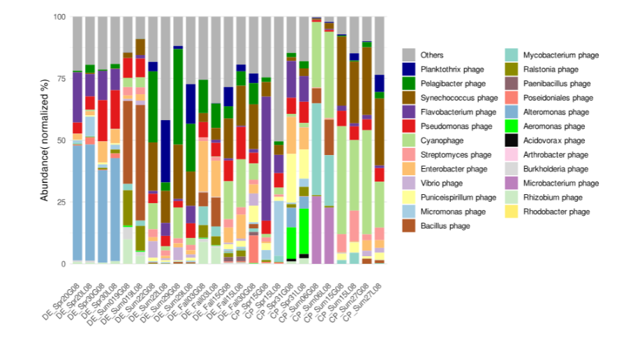
Part 8 — Quick visualisation ideas
Once you have the merged table, a few standard plots communicate the results clearly:
Stacked bar chart of relative abundance by taxonomy
import pandas as pd
import matplotlib.pyplot as plt

df = pd.read_csv("taxonomy_abundance_combined.tsv", sep="\t")

# Collapse to family level, sum relative abundance per sample
family_abund = df.groupby("family")[sample_cols].sum()
family_abund.T.plot(kind="bar", stacked=True, figsize=(10, 6), colormap="tab20")
plt.ylabel("Relative abundance")
plt.xlabel("Sample")
plt.legend(bbox_to_anchor=(1.05, 1), loc="upper left", fontsize=8)
plt.tight_layout()
plt.savefig("family_abundance_barplot.pdf", dpi=150)
Heatmap of top 30 vOTUs
import seaborn as sns

top30 = df.nlargest(30, df[sample_cols].mean(axis=1).name)
sns.clustermap(
    top30[sample_cols],
    cmap="YlOrRd",
    figsize=(10, 12),
    yticklabels=top30["family"].values,
    standard_scale=0
)
plt.savefig("top30_vOTU_heatmap.pdf", dpi=150)
Alpha diversity (richness per sample)
# Count vOTUs present (relative abundance > 0) per sample
richness = (df[sample_cols] > 0).sum()
print(richness)
These are starting points. The companion repository includes a full day2/scripts/plot_taxonomy_abundance.py script that generates publication-ready versions of these figures.
Part 9 — Common questions and pitfalls
Q: Most of my vOTUs come back as “Unknown”. Is something wrong?
No. This is normal, especially in underexplored environments. A recent large-scale ocean virome study found that ~70% of vOTUs had no family-level classification. Unknown vOTUs are not failures — they represent novel viral diversity. Document them, note their abundance, and consider whether any are abundant enough to warrant deeper investigation.
Q: My mapping rates are very low (<0.1%). Should I be worried?
Not necessarily. Viral sequences are a small fraction of total environmental DNA, so most reads in a bulk metagenome come from bacteria and archaea. Mapping rates to viral references of 0.1–5% are typical. Very low rates (<0.01%) can sometimes indicate that your samples were not viral-enriched and the assembly recovered very few viral contigs to begin with — check the size of vOTUs.fa relative to your full assembly.
Q: Some vOTUs have extremely high relative abundance in one sample and zero in all others. Is that real?
Possibly. Viral populations can be highly dynamic — a lytic phage can cause a bloom in one sample that wipes out its host, resulting in extremely high viral abundance followed by a crash. Check the covered fraction for that vOTU in the high-abundance sample (should be close to 1.0 for a genuine bloom) and check whether the read depth is consistent across the genome (genuine signal tends to be relatively uniform; false positives often show spiky coverage).
Q: Should I use relative_abundance or mean coverage for downstream statistics?
For between-sample comparisons, use relative_abundance — it accounts for differences in sequencing depth between samples. For within-sample comparisons of viral replication activity, mean coverage can be informative. For ordination (PCoA, NMDS) and diversity analyses, use relative_abundance.
What we have built
At the end of this post you have a complete taxonomy + abundance characterisation of your viral community:
| File | Contents |
|---|---|
genomad_output/vOTUs_summary/vOTUs_virus_summary.tsv | geNomad taxonomy and scores |
blastp_vs_refseq.txt | raw BLAST hits |
master_taxonomy.tsv | reconciled taxonomy from both methods |
*_sorted.bam | read mappings per sample |
coverm_abundance_all_samples.tsv | raw abundance matrix |
coverm_abundance_filtered.tsv | abundance matrix after coverage filter |
taxonomy_abundance_combined.tsv | merged final table |
In the next post we shift from who the viruses are to what they do — identifying auxiliary metabolic genes (AMGs) and understanding how viruses reshape host metabolism mid-infection.
Companion repository: metagenome-to-viromics Scripts, toy data, and install guides for every step in this series live here. Day 2 materials are in
day2/.