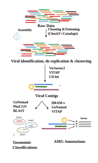
From Metagenome to Viral OTUs: Identifying, Filtering, and Clustering Viral Genomes
Part 1 — Why Viromics?
🧬 𝐷𝑎𝑦 78 𝑜𝑓 𝐷𝑎𝑖𝑙𝑦 𝐵𝑖𝑜𝑖𝑛𝑓𝑜𝑟𝑚𝑎𝑡𝑖𝑐𝑠 𝑓𝑟𝑜𝑚 𝐽𝑜𝑗𝑦’𝑠 desk
The invisible majority
When microbiologists talk about a microbiome — whether from the ocean, soil, or a human gut — they usually mean the bacteria and archaea. But there is an entire parallel community that rarely makes it onto the plot: the viruses.
In any spoonful of seawater, viral particles outnumber bacterial cells by roughly ten to one. In soil and sediment, the ratio is similar. These are not passive bystanders. Viruses infect and lyse microbial cells, releasing nutrients and carbon back into the environment in a process sometimes called the viral shunt. They transfer genes between hosts through transduction, accelerating microbial evolution. And a surprising number of them carry auxiliary metabolic genes (AMGs) — functional copies of host metabolic genes that the virus expresses during infection to boost its own replication, effectively reprogramming the host cell’s biochemistry mid-infection.
In short, you cannot fully understand a microbial ecosystem without understanding its viruses.
Why viruses are hard to detect
Bacteria and archaea have a universal marker gene — the 16S rRNA gene — that makes community profiling relatively straightforward. Amplify it, sequence it, count it.
Viruses have no such universal marker. They are phenomenally diverse, evolve rapidly, and share very few genes across groups. This means the only reliable way to detect them is to look at the raw sequence data itself: assemble the metagenome into contigs, then ask which contigs look viral.
This is the core challenge of viromics, and it is what this post walks through end to end.
The six-post series at a glance
| Post | Topic |
|---|---|
| 1 (this post) | Metagenome context, viral identification (VirSorter2 + VITAP), vOTU clustering, CheckV quality |
| 2 | Taxonomic classification (geNomad + BLAST) and abundance estimation (CoverM) |
| 3 | Auxiliary metabolic genes with DRAM-v |
| 4 | Host prediction with iPHoP |
| 5 | Viral lifestyle prediction (PhaBOX2) and network analysis (vConTACT2) |
| 6 | Active viral communities from metatranscriptomes and expressed AMGs |
Part 2 — Starting Point: The Assembled Metagenome
A metagenome is the collective DNA extracted from an environmental sample and sequenced without culturing. You homogenize the sample, extract total DNA, fragment it, and sequence millions of short paired-end reads. Those reads represent every organism present: bacteria, archaea, viruses, eukaryotes, and free-floating environmental DNA.
The first computational step is assembly — reconstructing longer contiguous sequences (contigs) from overlapping short reads using tools like MEGAHIT or metaSPAdes.
This series starts from already-assembled contigs. If you still need to assemble, a standard MEGAHIT run looks like this:
# Quality trim first (always worth doing)
fastp \
  -i sample_R1.fastq.gz -I sample_R2.fastq.gz \
  -o sample_R1_trimmed.fastq.gz -O sample_R2_trimmed.fastq.gz \
  --thread 16 --detect_adapter_for_pe

# Assemble
megahit \
  -1 sample_R1_trimmed.fastq.gz \
  -2 sample_R2_trimmed.fastq.gz \
  -o megahit_output \
  --min-contig-len 500 \
  -t 16
After assembly you will have one FASTA file containing hundreds of thousands of contigs — bacterial, archaeal, viral, and eukaryotic sequences all mixed together. The goal of everything that follows is to pull out the viral fraction.
Why viruses are hard to find inside a metagenome
Viral contigs tend to be shorter than bacterial ones (most viral genomes are 5–200 kb), their genes are highly divergent from cellular genes, and in bulk DNA extractions they are often under-represented because cellular DNA swamps them numerically. Two complementary approaches are needed to find them reliably:
- Machine learning on genome features — VirSorter2 learns patterns of gene density, coding strand bias, and viral hallmark gene content that distinguish viral from cellular contigs.
- Alignment-based taxonomy — VITAP translates contigs into predicted proteins, aligns them against a viral reference database, and assigns lineage. Contigs placed in Riboviria or Duplodnaviria are flagged as viral.
Running both and combining their output is standard practice. Each tool has complementary strengths and blind spots.
Part 3 — VirSorter2: Machine Learning Viral Prediction
VirSorter2 uses a combination of viral hallmark gene HMMs and a random forest classifier to score each contig for viral likelihood. It supports multiple viral groups: dsDNA phage, ssDNA viruses, RNA viruses, NCLDVs (giant viruses), and Lavidaviridae (virophages).
Environment setup
module load anaconda3/2023.09-0
conda activate /path/to/virsorter2_env
Running VirSorter2
virsorter run \
  -i assembly.fa \
  -w virsorter2_output \
  --db-dir /path/to/virsorter2_db \
  --min-length 1500 \
  --include-groups "dsDNAphage,ssDNA,RNA,NCLDV,lavidaviridae" \
  -j 16 \
  all
Key parameters explained:
| Parameter | What it does |
|---|---|
--min-length 1500 | ignore contigs shorter than 1500 bp — too short to reliably classify |
--include-groups | viral categories to screen for; include all unless you have a reason to exclude |
-j 16 | threads |
all | run the full pipeline including score calculation |
Key output file
virsorter2_output/final-viral-combined.fa
This FASTA contains all contigs that passed VirSorter2’s viral score threshold. This is the file you carry forward.
Note for DRAM-v users (Day 3): If you plan to run DRAM-v for AMG identification, you need to rerun VirSorter2 with
--prep-for-dramvadded to the command. This generates additional annotation files that DRAM-v requires. We cover this in the AMG post.
Part 4 — VITAP: Alignment-Based Viral Detection
VITAP predicts open reading frames on each contig and aligns the translated proteins against a curated viral reference database using DIAMOND. It assigns a taxonomic lineage to every contig, including reference genomes from the ICTV database alongside your sample contigs.
Environment setup
conda activate /path/to/VITAP_env
module load diamond/2.0.14
If VITAP has an older bundled DIAMOND version that conflicts with the module, resolve it before running:
ENV=/path/to/VITAP_env
mv "$ENV/bin/diamond" "$ENV/bin/diamond.old_0.9.19" 2>/dev/null || true
hash -r
module load diamond/2.0.14
which diamond    # should point to the module version
diamond version
Running VITAP
VITAP assignment \
  -i assembly.fa \
  -d /path/to/VITAP_db \
  -o vitap_output
Filtering viral contigs from VITAP output
VITAP assigns taxonomy to all contigs — it does not output a viral-only FASTA directly. You need to filter it yourself.
In this dataset, viral sequences belong to two realms: Riboviria (RNA viruses) and Duplodnaviria (dsDNA viruses including most phages).
Step 1 — inspect the output
head -n 5 vitap_output/best_determined_lineages.tsv
The file has four columns: Genome_ID, lineage, lineage_score, Confidence_level. IDs starting with k141_ are your assembled contigs; alphanumeric IDs like AJ428555.1 are ICTV reference genomes bundled in the database.
Step 2 — extract viral contig IDs
awk -F '\t' 'NR>1 && ($2 ~ /Riboviria|Duplodnaviria/) {print $1}' \
  vitap_output/best_determined_lineages.tsv > viral_ids.txt

wc -l viral_ids.txt
Step 3 — remove reference genomes
grep "^k" viral_ids.txt > viral_ids_clean.txt
wc -l viral_ids_clean.txt
Step 4 — extract sequences
module load seqkit

seqkit grep -f viral_ids_clean.txt \
  assembly.fa \
  > viral_contigs_vitap.fa

grep -c "^>" viral_contigs_vitap.fa   # should match wc -l viral_ids_clean.txt
Step 5 — optional length filter
For higher-confidence downstream analysis, filter to contigs ≥ 5 kb:
seqkit seq -m 5000 viral_contigs_vitap.fa > viral_contigs_vitap_min5kb.fa
Part 5 — Combining Both Tools
After running VirSorter2 and VITAP you have two viral FASTA files. Combining them captures the union of both detection strategies.
cat virsorter2_output/final-viral-combined.fa \
    viral_contigs_vitap_min5kb.fa \
    > viral_contigs_combined.fa
Because the two tools may have detected some of the same contigs, the combined file will contain duplicate sequences with different or identical headers. The clustering step below handles this, but if you want a clean deduplicated FASTA before clustering, the companion Python script combine_viral_contigs.py (in the repository) does this properly — it tracks which tool detected each contig, removes exact duplicates, and writes a summary table.
python scripts/combine_viral_contigs.py \
  --virsorter virsorter2_output/final-viral-combined.fa \
  --vitap viral_contigs_vitap_min5kb.fa \
  --out viral_contigs_combined.fa \
  --summary combine_summary.tsv
Part 6 — Clustering into vOTUs with CD-HIT
Individual viral contigs from different samples, or from different tools, may represent the same viral genome at slightly different coverage or with minor assembly errors. Clustering groups these into viral operational taxonomic units (vOTUs) — one representative per distinct viral genome.
The community standard for vOTU clustering is 95% nucleotide identity over 85% of the shorter contig’s length, following the Minimum Information about an Uncultivated Virus (MIUViG) guidelines.
module load cd-hit/4.8.1

cd-hit-est \
  -i viral_contigs_combined.fa \
  -o vOTUs.fa \
  -c 0.95 \
  -aS 0.85 \
  -T 20 \
  -M 0
Parameter reference:
| Parameter | Value | Meaning |
|---|---|---|
-c | 0.95 | 95% nucleotide identity threshold |
-aS | 0.85 | 85% alignment coverage of the shorter sequence |
-T | 20 | threads |
-M | 0 | unlimited memory usage |
The output vOTUs.fa contains one representative contig per cluster. This file is the input for all downstream steps in this series.
Part 7 — Quality Assessment with CheckV
Not all contigs in vOTUs.fa are complete viral genomes. Some are fragments, and some may carry host contamination (cellular DNA dragged along with a prophage). CheckV estimates genome completeness, detects contamination, and assigns a quality tier to each vOTU.
conda activate checkv_env

checkv end_to_end \
  vOTUs.fa \
  checkv_output \
  -d /path/to/checkv_db \
  -t 16
Key output files
| File | What it contains |
|---|---|
checkv_output/quality_summary.tsv | completeness, contamination, quality tier per vOTU |
checkv_output/viruses.fna | predicted free-living viral genomes |
checkv_output/proviruses.fna | viral regions integrated in host scaffolds |
checkv_output/contamination.tsv | detailed contamination estimates |
Quality tiers
| Tier | Completeness |
|---|---|
| Complete | circular or DTR-confirmed complete genome |
| High quality | ≥ 90% complete |
| Medium quality | 50–90% complete |
| Low quality | < 50% complete |
| Not determined | insufficient information |
For most downstream analyses — taxonomy, abundance, AMG identification — medium quality and above is a reasonable minimum. For network analysis and host prediction, high quality or complete genomes give the most reliable results.
Proviruses vs free-living viruses
CheckV distinguishes two types of viral sequences:
- Free-living viruses (
viruses.fna) — contigs that appear to be standalone viral genomes not integrated in a host - Proviruses (
proviruses.fna) — viral sequences embedded within a longer host scaffold; CheckV trims the host flanking regions
For most ecological analyses you will work with viruses.fna. Proviruses are important for understanding lysogeny (covered in Post 5) and should not be discarded.
Part 8 — What You Have at the End of This Step
After running through this pipeline you have:
-
vOTUs.fa— representative viral genomes, one per cluster, ready for taxonomy and abundance estimation -
checkv_output/quality_summary.tsv— quality metadata for every vOTU -
checkv_output/viruses.fna— free-living subset -
checkv_output/proviruses.fna— integrated prophage subset -
combine_summary.tsv— which tool detected each contig (useful for understanding detection overlap)
In the next post we assign taxonomy to these vOTUs using geNomad and BLAST, and estimate their abundance across samples using CoverM.
Companion repository: metagenome-to-viromics Toy assembly, batch scripts, the combine Python script, and installation guides for every tool used here.