Pangenomes, Biosynthetic Potential, and Population Structure: A Population Genomics Workflow
🧬 𝐷𝑎𝑦 𝟪7 𝑜𝑓 𝐷𝑎𝑖𝑙𝑦 𝐵𝑖𝑜𝑖𝑛𝑓𝑜𝑟𝑚𝑎𝑡𝑖𝑐𝑠 𝑓𝑟𝑜𝑚 𝐽𝑜𝑗𝑦’𝑠 𝖽𝖾𝗌𝗄
Two strains of the same bacterial species can look identical at the 16S level and yet carry fundamentally different genetic toolkits. One might produce an antimicrobial peptide that its close relatives cannot. Another might carry a unique cluster of metabolic genes that lets it colonize a niche that is hostile to every other member of its species. This is the core insight behind pangenome analysis: the genome of a species is not a fixed thing. It is a distributed archive, spread across all strains, containing a shared core and a vast accessory space that defines individual and population-level differences.
This post documents a complete population genomics workflow applied to Staphylococcus capitis — a coagulase-negative staphylococcus found on human skin and a clinically relevant opportunistic pathogen in neonatal intensive care units. The workflow moves from raw GenBank files through pangenome construction, population-specific gene enrichment, secondary metabolite prediction, and gene cluster family analysis. Where results from the ongoing study are not yet published, I use simplified toy examples to illustrate what each step produces and why it matters.
Why pangenomics? The core–accessory framework
Imagine you have genome sequences for 100 strains of the same species. You could align them all and look for single-nucleotide polymorphisms — that is phylogenomics. But pangenomics asks a different question: which genes are shared by all strains, which are shared by some, and which appear in only one or two? That partition is biologically meaningful.
A simplified toy example with five hypothetical strains:
| Gene cluster | Strain A | Strain B | Strain C | Strain D | Strain E | Frequency |
|---|---|---|---|---|---|---|
| GC_001 (ribosomal protein) | ✓ | ✓ | ✓ | ✓ | ✓ | 100% → Core |
| GC_002 (cell wall synthesis) | ✓ | ✓ | ✓ | ✓ | ✓ | 100% → Core |
| GC_003 (siderophore) | ✓ | ✓ | ✓ | ✗ | ✗ | 60% → Accessory |
| GC_004 (bacteriocin) | ✓ | ✗ | ✗ | ✗ | ✗ | 20% → Rare |
The core genome encodes the machinery every strain needs to survive. The accessory genome encodes everything that makes one strain different from another — virulence factors, resistance genes, metabolic specializations, biosynthetic gene clusters.
In a real dataset of 228 S. capitis genomes, the pangenome expands to thousands of gene clusters distributed across core, accessory, low-frequency, and rare categories. The proportion that is core typically shrinks as more genomes are added — a hallmark of an open pangenome, which suggests ongoing horizontal gene transfer and ecological diversification.
Project structure and inputs
/scratch/jojyj/capitis_work/
├── capitis_GenBank/     # input: annotated genome files (.gbk)
├── fasta/               # converted FASTA sequences
├── contigs_db/          # anvi'o contigs databases
├── pan_output/          # anvi'o pangenome database
├── exports/             # gene cluster tables
├── antismash_output/    # per-genome BGC predictions
├── bgc_summary/         # aggregated BGC tables
└── bigscape_input/      # antiSMASH region files for BiG-SCAPE
The metadata assigns each genome to one of seven phylogenomic populations (SC_pop_1 through SC_pop_7), defined based on prior phylogenetic analysis. These population labels drive the enrichment analysis downstream.
Step 1 — Convert GenBank to FASTA
anvi’o requires FASTA input. The GenBank files from NCBI contain both sequence and annotation, so the conversion extracts the sequence while keeping contig names consistent:
from Bio import SeqIO
import glob, os

gbk_dir = "capitis_GenBank"
out_dir = "fasta"
os.makedirs(out_dir, exist_ok=True)

for gbk in glob.glob(f"{gbk_dir}/*.gbk"):
    sample = os.path.basename(gbk).replace(".gbk", "")
    sample = sample.replace(" ", "_").replace("-", "_").replace(".", "_")
    out = f"{out_dir}/{sample}.fa"

    with open(out, "w") as handle:
        for i, record in enumerate(SeqIO.parse(gbk, "genbank"), start=1):
            record.id          = f"{sample}_contig_{i}"
            record.name        = record.id
            record.description = ""
            SeqIO.write(record, handle, "fasta")
The renaming step — replacing spaces, hyphens, and dots with underscores — matters downstream. anvi’o is strict about special characters in genome names, and a mismatch between the name in the FASTA and the name used elsewhere in the pipeline will cause silent failures that are hard to trace.
Step 2 — Build the anvi’o pangenome
anvi’o pangenomics works in four stages: build per-genome contigs databases, run COG annotation on each, merge them into a genomes storage, then run the pangenome analysis.
conda activate anvio-9

# Per-genome contigs databases
for fa in fasta/*.fa; do
    sample=$(basename "$fa" .fa)
    anvi-gen-contigs-database -f "$fa" -o contigs_db/${sample}.db -n "$sample" --num-threads 8
done

# COG functional annotation
for db in contigs_db/*.db; do
    anvi-run-ncbi-cogs -c "$db" --num-threads 8
done

# External genomes manifest
echo -e "name\tcontigs_db_path" > external-genomes.txt
for db in contigs_db/*.db; do
    sample=$(basename "$db" .db)
    echo -e "${sample}\t$(realpath "$db")" >> external-genomes.txt
done

# Genomes storage
anvi-gen-genomes-storage -e external-genomes.txt -o STAPH_CAPITIS-GENOMES.db

# Pangenome
anvi-pan-genome \
    -g STAPH_CAPITIS-GENOMES.db \
    -n STAPH_CAPITIS_PAN \
    -o pan_output \
    --num-threads 16 \
    --minbit 0.5 \
    --mcl-inflation 10 \
    --I-know-this-is-not-a-good-idea
The last flag — --I-know-this-is-not-a-good-idea — is required when the genome count exceeds anvi’o’s recommended limit. It is not a workaround; it is an explicit acknowledgment that computing the all-vs-all BLAST matrix for hundreds of genomes is computationally expensive and that the user accepts responsibility for the resource implications. The analysis is still statistically valid.
--minbit 0.5 sets the minimum bit score ratio for retaining BLAST hits, controlling sensitivity. --mcl-inflation 10 controls how tightly the Markov clustering algorithm groups similar sequences — higher inflation produces more, smaller, tighter gene clusters.
Step 3 — Gene presence–absence matrix
After exporting gene clusters, the raw table is converted into a binary presence–absence matrix. This is the input for everything downstream — enrichment testing, visualization, and any ecological analysis.
import pandas as pd

df = pd.read_csv("exports/gene_clusters.txt", sep="\t")

gc_col     = [c for c in df.columns if "gene_cluster" in c][0]
genome_col = [c for c in df.columns if "genome" in c][0]

pa = (
    df[[gc_col, genome_col]]
    .drop_duplicates()
    .assign(present=1)
    .pivot_table(index=gc_col, columns=genome_col, values="present", fill_value=0)
)
For each gene cluster, this matrix records 1 (present) or 0 (absent) across every genome. The frequency column — how many genomes carry a given cluster — drives the core/accessory categorization:
| Frequency threshold | Category |
|---|---|
| ≥ 95% | Core |
| 15–95% | Accessory |
| 5–15% | Low-frequency accessory |
| < 5% | Rare |
These thresholds are conventional, not universal. For a tightly clonal species with limited horizontal gene transfer, you might raise the core threshold. For a highly diverse species, you might lower it. The biological question should guide the cutoffs.
Step 4 — Metadata alignment and name matching
A recurrent practical challenge in pangenomics is that genome names in the presence–absence matrix and genome names in the metadata rarely match perfectly. NCBI GenBank names include strain designations, subspecies annotations, and version suffixes that differ from the clean names used in the metadata spreadsheet.
The fix is a systematic matching pipeline: check which names are present in both, use fuzzy matching to identify likely pairs for unmatched names, build a correction table manually for ambiguous cases, then apply corrections and merge.
from difflib import get_close_matches

missing = sorted(set(pa_names) - set(meta_names))

for m in missing:
    matches = get_close_matches(m, meta_names, n=5, cutoff=0.4)
    print(f"PA name: {m}")
    for x in matches:
        print(f"  → candidate: {x}")
For example:
PA name: Staphylococcus_capitis_subsp__capitis_strain_DE0241
  → candidate: Staphylococcus_capitis_strain_DE0241
The correction is obvious once surfaced, but impossible to catch without running the check first. Running all(pa_names %in% meta_names) before every downstream step is non-negotiable.
Step 5 — Population-specific gene enrichment
Once metadata is aligned, the enrichment analysis asks: for each gene cluster and each population, is that cluster significantly more prevalent in this population than in all others combined? This is a 2×2 Fisher’s exact test for every gene cluster × population combination.
To illustrate with a toy example — imagine gene cluster GC_042 appears in 45 of 50 SC_pop_3 genomes (90%) but only in 12 of 178 genomes from all other populations combined (7%):
                 GC_042 present   GC_042 absent
SC_pop_3              45               5
All others            12             166

Fisher's exact test: p < 0.0001, OR = 124, frequency difference = +0.83
That cluster is strongly enriched in SC_pop_3. Something in the biology of this lineage favors carrying this gene — whether it is positive selection, a founder effect, or a shared ecological niche would require further investigation.
The R implementation runs this test for every gene cluster in every population:
library(tidyverse)

results <- list()

for (target in unique(meta$clade)) {

  res <- pa_long %>%
    mutate(in_target = clade == target) %>%
    group_by(gene_cluster) %>%
    summarise(
      target_present = sum(present == 1 & in_target),
      target_absent  = sum(present == 0 & in_target),
      other_present  = sum(present == 1 & !in_target),
      other_absent   = sum(present == 0 & !in_target),
      .groups = "drop"
    ) %>%
    rowwise() %>%
    mutate(
      fisher = list(fisher.test(matrix(
        c(target_present, target_absent, other_present, other_absent), nrow = 2
      ))),
      pvalue     = fisher$p.value,
      odds_ratio = as.numeric(fisher$estimate)
    ) %>%
    ungroup() %>%
    select(-fisher) %>%
    mutate(
      clade                = target,
      target_frequency     = target_present / (target_present + target_absent),
      other_frequency      = other_present  / (other_present  + other_absent),
      frequency_difference = target_frequency - other_frequency,
      qvalue               = p.adjust(pvalue, method = "BH"),
      log2_odds_ratio      = log2(odds_ratio)
    )

  results[[target]] <- res
}

all_results <- bind_rows(results)

sig <- all_results %>%
  filter(
    qvalue < 0.05,
    odds_ratio > 1,
    target_frequency >= 0.50,      # present in at least half the target population
    frequency_difference >= 0.30   # at least 30 percentage points more common
  )
The four-condition filter for significance is important. Statistical significance alone (qvalue < 0.05) is not enough — a gene cluster that is present in 3% of one population and 0.5% of another can be highly significant with enough genomes, but is biologically uninterpretable as a population marker. The frequency and frequency-difference filters enforce biological relevance alongside statistical confidence.
Step 6 — Visualizing enrichment: volcano plots
A volcano plot of log₂(odds ratio) vs. −log₁₀(FDR) shows the enrichment landscape for each population simultaneously. Points to the right represent gene clusters that are more prevalent in the target population; points above the dashed significance line passed the FDR threshold.
vol_plot <- all_results %>%
  filter(target_frequency > 0.2 | other_frequency > 0.2) %>%
  mutate(
    significant  = qvalue < 0.05 & odds_ratio > 1 &
                   target_frequency >= 0.50 & frequency_difference >= 0.30,
    neglog10q    = -log10(qvalue)
  ) %>%
  filter(is.finite(log2_odds_ratio), is.finite(neglog10q))

ggplot(vol_plot, aes(x = log2_odds_ratio, y = neglog10q, color = significant)) +
  geom_point(size = 1.4, alpha = 0.75) +
  facet_wrap(~clade, scales = "free_y", ncol = 2) +
  scale_color_manual(values = c("FALSE" = "grey75", "TRUE" = "#D73027")) +
  geom_hline(yintercept = -log10(0.05), linetype = "dashed", linewidth = 0.3) +
  theme_bw(base_size = 14) +
  labs(
    x = expression(log[2]("Odds ratio")),
    y = expression(-log[10]("FDR")),
    color = NULL
  )
The faceted layout lets you compare populations directly. A population with many red points carries a highly differentiated accessory genome. A population with few red points shares most of its gene content with others — suggesting recent divergence, or that it is a generalist without strong niche-specific adaptations.
Step 7 — Secondary metabolite prediction with antiSMASH
The pangenome tells you which genes are present and where. antiSMASH tells you whether any of those genes are organized into biosynthetic gene clusters — coordinated sets of genes that together produce a secondary metabolite.
Secondary metabolites are ecologically and clinically significant: they include antibiotics, siderophores (iron-scavenging compounds), quorum-sensing signals, and antimicrobial peptides like lanthipeptides. For a skin commensal like S. capitis, these molecules may mediate competition with S. aureus and other pathogens in the skin niche.
# Run antiSMASH for all genomes
for gbk in capitis_GenBank/*.gbk; do
    sample=$(basename "$gbk" .gbk)
    antismash "$gbk" \
        --output-dir "antismash_output/$sample" \
        --genefinding-tool none \
        --cpus 16 \
        --cb-general \
        --cb-subclusters \
        --cb-knownclusters \
        --asf \
        --pfam2go \
        --smcog-trees
done
--genefinding-tool none tells antiSMASH to use the existing annotation in the GenBank file rather than re-predict genes. This is essential when working with NCBI-annotated genomes — re-predicting genes from scratch can produce different gene models that conflict with the annotation used in the pangenome analysis.
What antiSMASH identifies
For each genome, antiSMASH scans for signature biosynthetic genes and reports predicted BGC regions. Each region gets assigned to a BGC class. Some common classes in staphylococci:
| BGC class | What it makes | Biological role |
|---|---|---|
| lanthipeptide | Lanthipeptides (e.g., epidermin) | Antimicrobial peptides |
| NI-siderophore | Staphyloferrin-type siderophores | Iron acquisition |
| NRPS / NRPS-like | Non-ribosomal peptides | Diverse — antibiotics, siderophores, surfactants |
| T3PKS | Type III polyketides | Pigments, signaling molecules |
| terpene / terpene precursor | Terpene-derived compounds | Membrane components, signaling |
| cyclic lactone autoinducer | RNAIII-type quorum sensing signals | Density-dependent gene regulation |
Step 8 — Aggregating BGCs across all genomes
antiSMASH produces one output folder per genome, each containing region-level GenBank files. The summarization step extracts BGC class annotations from all regions across all genomes into a single table:
import os, glob, pandas as pd
from Bio import SeqIO

rows = []

for f in glob.glob("antismash_output/*/*.region*.gbk"):
    genome = os.path.basename(os.path.dirname(f))
    record = SeqIO.read(f, "genbank")

    bgc_classes = []
    for feature in record.features:
        if feature.type == "region":
            bgc_classes.extend(feature.qualifiers.get("product",
                               feature.qualifiers.get("region_type", ["unknown"])))

    for bgc_class in bgc_classes:
        rows.append({"genome": genome, "bgc_class": bgc_class.replace("-",".")})

df = pd.DataFrame(rows)
This produces a long-format table: one row per genome × BGC region. From this, you can derive a BGC class presence–absence matrix and classify each class as core, accessory, or rare using the same prevalence thresholds as the gene cluster analysis.
A core BGC class (present in ≥95% of genomes) is part of the essential metabolic toolkit of the species — likely under purifying selection. An accessory BGC class (present in 15–95%) is maintained in some lineages and may reflect niche adaptation or ongoing horizontal gene transfer.
Step 9 — BGC prevalence by population
With BGC presence–absence data and population metadata aligned, you can ask: does the biosynthetic potential of S. capitis differ between populations? Do some lineages carry more antimicrobial peptide biosynthetic clusters? Are siderophore clusters enriched in populations from iron-limited environments?
bgc_prev <- bgc_long %>%
  group_by(clade, bgc_class) %>%
  summarise(
    prevalence       = mean(present),
    genomes_present  = sum(present),
    .groups = "drop"
  )

ggplot(bgc_prev_plot, aes(x = clade, y = prevalence, fill = bgc_class)) +
  geom_col(position = position_dodge(width = 0.9), width = 0.8) +
  scale_fill_manual(values = bgc_colors) +
  theme_bw(base_size = 14) +
  labs(x = "Population", y = "BGC prevalence", fill = "BGC class")
The population-level BGC enrichment statistics use the same Fisher’s exact test framework as the gene cluster enrichment, but applied to BGC class presence–absence rather than gene cluster presence–absence. Significant enrichment of a BGC class in a specific population is a hypothesis-generating finding: it suggests that lineage-specific secondary metabolite production may contribute to whatever distinguishes that population ecologically or clinically.
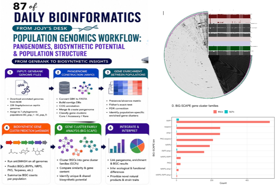
Step 10 — Gene cluster family analysis with BiG-SCAPE
antiSMASH predicts BGCs independently for each genome. Two genomes might each carry a lanthipeptide cluster, but are they the same lanthipeptide cluster or different ones that evolved separately? BiG-SCAPE answers this by comparing all BGC regions across all genomes and clustering them into Gene Cluster Families (GCFs) based on sequence similarity.
# Collect all antiSMASH region files
find antismash_output -name "*region*.gbk" -exec cp {} bigscape_input/ \;

# Run BiG-SCAPE
bigscape cluster \
    -i bigscape_input \
    -o bigscape_output \
    --mix
The output groups BGCs into families. A large GCF with members from many strains is a conserved, widespread biosynthetic pathway. A small GCF with members from only a few closely related strains may represent a recently acquired or actively diversifying pathway.
To illustrate with a toy example: imagine you have 10 genomes, each predicted to carry a “lanthipeptide” cluster by antiSMASH. BiG-SCAPE might group them like this:
GCF_001: 8 genomes — conserved epidermin-like cluster (core)
GCF_002: 2 genomes — divergent lanthipeptide, potentially novel
GCF_001 is the expected core pathway. GCF_002 is the interesting one — two strains carrying a divergent variant worth characterizing further.
The distribution of BGCs into GCFs, stratified by biosynthetic category and by population, gives the most detailed view of biosynthetic diversity available from comparative genomics alone.
Putting it together: the manuscript figure plan
The workflow produces two main figures:
Figure 1 — Population-specific accessory genome differentiation
- 1A: Phylogenetic tree colored by population
- 1B: Volcano plots of population-enriched gene clusters (one panel per population)
- 1C: Heatmap of top enriched gene clusters, samples ordered by population
Figure 2 — Secondary metabolite and BGC diversity
- 2A: BGC class prevalence across all genomes, colored by core/accessory/rare
- 2B: BGC class prevalence broken down by population (grouped bar chart)
Together, these figures tell a coherent story: the seven S. capitis populations are not just phylogenetically distinct — they carry different functional gene repertoires (Figure 1) and different biosynthetic potentials (Figure 2). Whether those differences are adaptive, neutral, or clinically meaningful is the next question.
What this analysis can and cannot tell you
A pangenome enrichment analysis identifies which gene clusters are statistically associated with a population. It does not tell you:
- Whether those genes are expressed (that requires transcriptomics)
- Whether the encoded proteins are functional (that requires biochemistry or functional genomics)
- Whether the association is causal or correlative (that requires experimental manipulation or natural experiments)
- What the gene clusters actually do, unless they match a characterized reference
The BGC analysis adds a layer: antiSMASH predictions are based on sequence similarity to characterized biosynthetic pathways. A predicted lanthipeptide cluster in S. capitis may or may not produce the same compound as the reference lanthipeptide used to train the model. Validation — heterologous expression, metabolomics, bioactivity assays — is required before any BGC prediction becomes a biological claim.
This is the honest framing of comparative genomics: it generates hypotheses at scale. The experiments that test those hypotheses are a separate undertaking.
Reproducibility checklist
- Genome names are standardized before any anvi’o step — no spaces, hyphens, or special characters.
-
all(pa_names %in% meta_names)returns TRUE before enrichment analysis. - COG annotation is confirmed to have run successfully for all contigs databases before pangenome generation.
-
--genefinding-tool noneused in antiSMASH when input files carry existing annotations. - Fisher’s exact test results are filtered on both statistical (FDR < 0.05) and biological (frequency ≥ 0.50, frequency difference ≥ 0.30) criteria.
-
sessionInfo()saved alongside all R output. - All Python scripts and SLURM submission scripts versioned alongside the result files.
This post documents an ongoing study. Results described here are preliminary and subject to change. antiSMASH version used: current conda-forge/bioconda release. anvi’o version: 9. BiG-SCAPE: current release. Population assignments based on prior phylogenomic analysis.