Beyond Expression: Normalizing Metatranscriptomic Signal with MTXmodel

🧬 𝐷𝑎𝑦 85 𝑜𝑓 𝐷𝑎𝑖𝑙𝑦 𝐵𝑖𝑜𝑖𝑛𝑓𝑜𝑟𝑚𝑎𝑡𝑖𝑐𝑠 𝑓𝑟𝑜𝑚 𝐽𝑜𝑗𝑦’𝑠 desk

A gene that is highly transcribed in a community might just be highly abundant in the community’s DNA. If a microbe with a given metabolic gene doubles in population, its RNA output doubles too — even if transcription per cell stays flat. Standard differential expression tools like DESeq2 treat every gene independently and normalize across samples, but they do not account for this feature-level confounding. MTXmodel does. This post covers why the adjustment matters, how the tool works, and a complete R workflow for applying it to estuarine metatranscriptomic data across salinity, season, and bay gradients.

The core problem: RNA abundance is not the same as transcriptional response

Imagine two samples. In sample A, a sulfur oxidation gene has 1,000 RNA reads and 100 DNA copies per cell. In sample B, the same gene has 2,000 RNA reads and 200 DNA copies per cell. The RNA doubled — but so did the gene abundance. The transcription rate per gene copy is identical. A naive differential expression test flags this as significant. MTXmodel does not, because it adjusts for the DNA abundance of each feature as a continuous covariate in the linear model.

This is the core idea behind the approach described in Zhang et al. (2021, Bioinformatics): incorporate feature-specific DNA abundance directly into the association model so that detected RNA changes reflect regulation, not population shifts.

A significant RNA change after MTXmodel adjustment is evidence of a transcriptional response. Without the adjustment, it could just be a bloom.

Installation

The package lives on GitHub and installs cleanly via devtools:

library(devtools)
install_github('biobakery/MTX_model')

MTXmodel is built on MaAsLin2 and inherits all of its model infrastructure — linear models, CPLM, negative binomial, zero-inflated — along with its normalization and transformation options. The key addition is the input_dnadata argument, which feeds per-feature DNA abundance into each feature’s model as a covariate.

The current workflow here uses MaAsLin 3 (the successor), which shares the same input structure but has updated model fitting and output formatting.

Input files: what you need and where it comes from

MTXmodel requires three files. All three must share the same feature IDs and the same sample IDs — alignment across all three is the first thing to verify before any modeling.

1. RNA abundance table

Features as rows, samples as columns. In this study, this comes from HUMAnN 2/3 pathway or gene output — the same pipeline that generates stratified community-level functional profiles. For MAG-based workflows, a similar table can be generated from read mapping back to predicted genes (e.g., via featureCounts or CoverM), which is worth exploring as an alternative to HUMAnN for genome-resolved metatranscriptomics.

             Sample_1   Sample_2   Sample_3 ...
nirS             1240        880       2100
dsrA              560        430        970
mcrA              210         90        440
...

2. DNA abundance table (the covariate)

Same dimensions, same feature IDs, same sample IDs — but from the metagenome rather than the metatranscriptome. This is the gene or pathway DNA abundance produced by HUMAnN 2/3 from the DNA fraction of the same samples. This table is what makes MTXmodel different from running MaAsLin on RNA alone.

3. Metadata file

Samples as rows, covariates as columns. Standard format shared with MaAsLin 2/3.

A note specific to estuarine data: MaAsLin was developed and validated primarily on human gut microbiome datasets, where metadata tends to be a handful of clinical or demographic variables (diagnosis, age, antibiotics). Estuarine datasets carry far more environmental covariates — salinity, season, bay, temperature, dissolved oxygen, chlorophyll, nutrient concentrations — and many of these are collinear. Feeding all of them into a single MaAsLin model inflates the multiple testing burden, reduces power, and can produce unstable coefficient estimates when predictors correlate.

The practical solution: keep the metadata design as sparse as possible. Run focused models — salinity within a bay, season as the only predictor — rather than trying to explain everything in a single omnibus model. Subset the data to relevant comparisons. This is not a limitation of the tool; it is sound statistical practice for high-dimensional environmental data.

Step 1 — Load and align data

library(MTXmodel)
library(maaslin3)

# Load data
df_rna  <- read.csv("MT_Sum.csv",      row.names = 1, check.names = FALSE)
df_dna  <- read.csv("MG_sum.csv",      row.names = 1, check.names = FALSE)
df_meta <- read.csv("metadata.csv",    row.names = 1, check.names = FALSE)

# Align samples across all three inputs
common_samples <- Reduce(intersect, list(
  colnames(df_rna),
  colnames(df_dna),
  rownames(df_meta)
))

df_rna  <- df_rna[, common_samples]
df_dna  <- df_dna[, common_samples]
df_meta <- df_meta[common_samples, ]

# Align features (genes/pathways) between RNA and DNA tables
common_features <- intersect(rownames(df_rna), rownames(df_dna))
df_rna <- df_rna[common_features, ]
df_dna <- df_dna[common_features, ]

# Confirm dimensions match
dim(df_rna)   # should be features × samples
dim(df_dna)   # should match df_rna exactly

The Reduce(intersect, ...) call is the critical step. Samples present in RNA but absent in DNA (or metadata) are silently dropped — this is expected and safe, but you should inspect common_samples to confirm no unexpected losses. If a large fraction of samples disappears here, that indicates a naming inconsistency between files (e.g., "Sample_1" vs "sample_1" vs "S1").

Step 2 — Set factor levels and reference groups

df_meta$Bay      <- factor(df_meta$Bay,      levels = c("CP", "Delaware"))
df_meta$Season   <- factor(df_meta$Season,   levels = c("Spring", "Summer"))
df_meta$Salinity <- factor(df_meta$Salinity, levels = c("Low", "Medium", "High"))

The first level in each factor() call becomes the reference group. All model coefficients are interpreted relative to these references: BayDelaware is Delaware vs. CP, SeasonSummer is Summer vs. Spring, SalinityMedium and SalinityHigh are both relative to Low. Explicit levels prevents alphabetical defaults from silently changing what the coefficients mean — the same principle as relevel() in DESeq2.

Step 3 — Global model: raw RNA abundances with MaAsLin 3

The first model tests all three factors simultaneously across all samples. This gives a broad view of which genes associate with bay, season, or salinity, but coefficient estimates for each factor are adjusted for the others.

library(maaslin3)

OUT_BASE <- "~/MTX_modeling_output"
dir.create(OUT_BASE, showWarnings = FALSE, recursive = TRUE)

out_rna <- file.path(OUT_BASE, "maaslin3_RNA")
dir.create(out_rna, showWarnings = FALSE, recursive = TRUE)

set.seed(1)

fit_maaslin_rna <- maaslin3(
  input_data      = df_rna,
  input_metadata  = df_meta,
  output          = out_rna,
  fixed_effects   = c("Bay", "Season", "Salinity"),
  random_effects  = NULL,
  normalization   = "NONE",
  transform       = "LOG"
)

normalization = "NONE" is correct here — the DNA covariate adjustment will handle the compositional normalization when MTXmodel is run. transform = "LOG" applies a log transformation to stabilize variance before linear modeling, which is the recommended default for count-like abundance data. set.seed(1) ensures reproducibility for any permutation-based steps in the model fitting.

The output folder will contain all_results.tsv with coefficients, standard errors, p-values, and q-values for every feature × metadata term combination.

Step 4 — Focused subset models for salinity within each Bay × Season

The global model tests salinity while adjusting for bay and season, but it cannot tell you whether the salinity effect is consistent across bays and seasons — or whether it only appears in one context. Subset models answer this directly:

run_subset_maaslin <- function(bay, season, out_name) {
  keep <- rownames(df_meta)[df_meta$Bay == bay & df_meta$Season == season]

  if (length(keep) < 3) {
    message("Not enough samples for: ", bay, " / ", season)
    return(NULL)
  }

  maaslin3(
    input_data     = df_rna[, keep, drop = FALSE],
    input_metadata = df_meta[keep, , drop = FALSE],
    output         = file.path(OUT_BASE, out_name),
    fixed_effects  = c("Salinity"),
    random_effects = NULL
  )
}

fit_CP_Summer <- run_subset_maaslin("CP",       "Summer", "maaslin3_RNA_CP_Summer_Salinity")
fit_CP_Spring <- run_subset_maaslin("CP",       "Spring", "maaslin3_RNA_CP_Spring_Salinity")
fit_DE_Summer <- run_subset_maaslin("Delaware", "Summer", "maaslin3_RNA_DE_Summer_Salinity")
fit_DE_Spring <- run_subset_maaslin("Delaware", "Spring", "maaslin3_RNA_DE_Spring_Salinity")

The length(keep) < 3 guard prevents the function from silently fitting a model with too few samples to estimate variance — a common source of nonsense results in subset analyses. If a particular Bay × Season combination has fewer than three samples, it gets skipped with a message rather than crashing or producing unreliable output.

Step 5 — Visualizing results

Coefficient plot

library(ggplot2)
library(readr)
library(dplyr)

res <- read_tsv(file.path(out_rna, "all_results.tsv"))

# Keep only significant associations (MaAsLin default q-value threshold: 0.25)
res_sig <- res %>% filter(qval < 0.25)

ggplot(res_sig, aes(x = coef, y = reorder(feature, coef), color = metadata)) +
  geom_point(size = 3) +
  geom_vline(xintercept = 0, linetype = "dashed") +
  labs(
    x     = "Coefficient (effect size)",
    y     = "Feature",
    color = "Metadata term",
    title = "MaAsLin 3: Raw RNA abundances"
  ) +
  theme_minimal(base_size = 12)

Each point is a significant feature × metadata term association. Points to the right of zero are positively associated with the non-reference level (e.g., higher RNA in Delaware vs. CP, or in Summer vs. Spring); points to the left are negatively associated. Color distinguishes which metadata variable is driving each association.

Heatmap of top features

library(pheatmap)

# Select top 50 most significant features across all terms
top_feats <- res_sig %>%
  arrange(qval) %>%
  slice_head(n = 50) %>%
  pull(feature)

mat <- df_rna[top_feats, colnames(df_rna) %in% rownames(df_meta)]
ann <- df_meta[, c("Bay", "Season", "Salinity"), drop = FALSE]

pheatmap(
  mat,
  annotation_col = ann,
  scale          = "row",
  show_rownames  = FALSE,
  main           = "Raw RNA Abundance — Top 50 Features"
)

scale = "row" converts each gene’s abundances to z-scores across samples, which lets you see relative patterns rather than absolute magnitudes. Without row-scaling, highly abundant genes dominate the color range and low-abundance features become invisible.

Step 6 — Running MTXmodel with DNA covariate adjustment

Once you have confirmed the global and subset MaAsLin models look reasonable, the full MTXmodel run adds the DNA covariate. This is the step that separates transcriptional regulation from gene copy number effects:

library(MTXmodel)

fit_mtx <- MTXmodel(
  input_data     = df_rna,
  input_metadata = df_meta,
  output         = file.path(OUT_BASE, "MTXmodel_output"),
  fixed_effects  = c("Bay", "Season", "Salinity"),
  random_effects = NULL,
  normalization  = "NONE",
  transform      = "LOG",
  standardize    = FALSE,
  input_dnadata  = df_dna,
  rna_dna_flt    = "semi_strict"
)

The rna_dna_flt argument controls which samples are retained for each feature’s model. The options range from none (no filtering) to strict (require both RNA and DNA detected in every sample). semi_strict — the recommended starting point — excludes samples where both the feature’s DNA and RNA are undetected, while retaining samples where one but not both is zero. This avoids fitting models on features that are absent across large swaths of the dataset while preserving real sparse-but-present signal.

Genes that show significant associations in the MTXmodel output but not in the raw MaAsLin RNA model (or vice versa) are particularly interesting: they represent cases where DNA-level confounding was masking or inflating the transcriptional signal.

What the output tells you — and what it does not

The default significance threshold in MaAsLin and MTXmodel is qval < 0.25, which is more permissive than the padj < 0.05 threshold commonly used in DESeq2. This reflects the discovery-oriented framing of MaAsLin — it is designed to identify candidate associations in complex microbiome datasets where effect sizes are typically smaller than in controlled transcriptomics experiments. For a publication, you will want to apply a stricter threshold or prioritize features that are significant across multiple subset models.

As with any association model in environmental data: a significant coefficient tells you that RNA abundance of a gene correlates with a metadata variable, after controlling for the other terms in the model and the DNA covariate. It does not tell you which organism is responding, what the downstream metabolic consequence is, or whether the association is causal. Those interpretations require additional evidence — genome-resolved analysis, targeted validation, or orthogonal datasets.

Reproducibility checklist

1. RNA and DNA tables contain the same features (rows) and samples (columns) after alignment.
2. Reduce(intersect, ...) result inspected — no unexpected sample losses.
3. Factor levels set explicitly with factor(..., levels = ...) before modeling.
4. set.seed(1) called before any MaAsLin / MTXmodel run.
5. normalization = "NONE" used with raw counts when DNA covariate adjustment is applied.
6. qval used for filtering, not pval.
7. Subset models run for each Bay × Season combination to test consistency of salinity effects.
8. rna_dna_flt argument documented — semi_strict recommended as default.
9. All output folders saved with descriptive names that encode the model specification.
10. sessionInfo() saved alongside results.

sessionInfo()

MTXmodel is developed by the Huttenhower Lab (biobakery/MTX_model). Cite: Zhang Y, Thompson KN, Huttenhower C, Franzosa EA. “Statistical approaches for differential expression analysis in metatranscriptomics.” Bioinformatics, 37(Suppl_1):i34–i41 (2021).

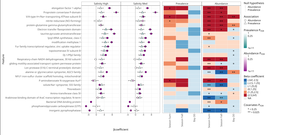
This MTXmodel plot below shows how microbial functional features associate with salinity, season, and bay after correcting for DNA abundance effects. The coefficient plots show the direction and strength of associations, while the heatmaps summarize statistical significance for feature abundance and prevalence across environmental gradients.