Day 5: Genome Annotation - Understanding Metabolic Potential
Day 5: Genome Annotation - Understanding Metabolic Potential
| Estimated Time: 6-10 hours | Difficulty: Intermediate | Prerequisites: Day 4 (Taxonomy) |
📚 Table of Contents
- Introduction
- Annotation Overview
- Software Installation
- Basic Annotation
- Advanced Annotation
- Metabolic Reconstruction
- Comparative Analysis
- Best Practices
- Troubleshooting
🎯 Introduction
Welcome to Day 5! You’ve recovered high-quality MAGs and classified them taxonomically. Now the exciting question: What can these organisms do?
Today’s goals:
- ✅ Predict genes - Where are the genes in your genomes?
- ✅ Assign functions - What do these genes do?
- ✅ Reconstruct pathways - What metabolic capabilities exist?
- ✅ Compare genomes - How do species differ functionally?
Why Annotate?
Unannotated genome: Just DNA sequences
Annotated genome: Blueprint of an organism’s capabilities
Answers you’ll get:
- Can it fix nitrogen?
- Does it produce secondary metabolites?
- What carbon sources can it use?
- Does it have antibiotic resistance genes?
- Can it degrade pollutants?
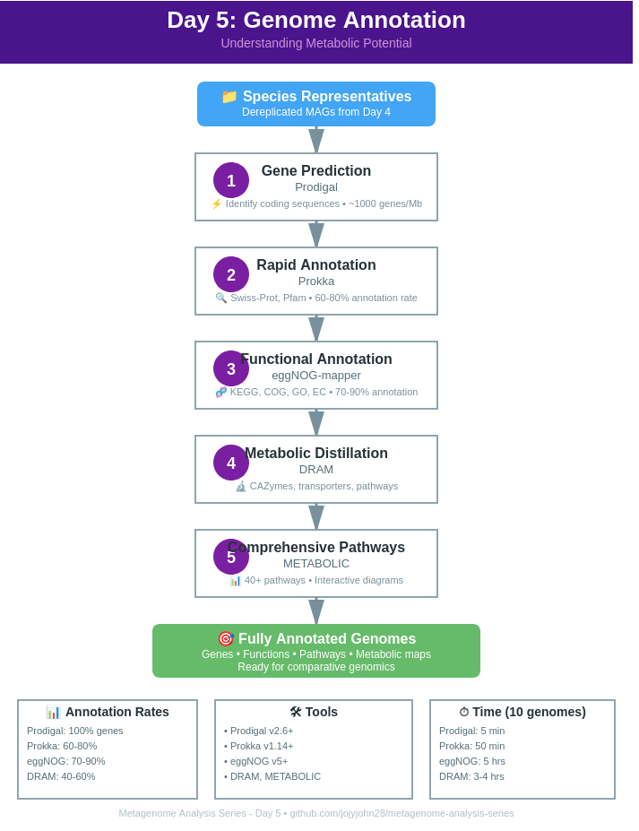
🔬 Annotation Overview
The Annotation Hierarchy
Level 1: Gene Prediction
├─ Prodigal    (Fast, accurate)
└─ Prokka      (Gene prediction + basic annotation)

Level 2: Functional Annotation
├─ eggNOG-mapper  (Orthology-based)
└─ Prokka         (Swiss-Prot, Pfam)

Level 3: Metabolic Annotation
├─ DRAM          (Metabolic distillation)
└─ METABOLIC     (Comprehensive pathways)
Tools Comparison
| Tool | Speed | Depth | Best For |
|---|---|---|---|
| Prodigal | ⚡⚡⚡ | Basic | Gene prediction only |
| Prokka | ⚡⚡ | Good | Quick annotation, publication |
| eggNOG-mapper | ⚡ | Excellent | Detailed functional annotation |
| DRAM | ⚡ | Excellent | Metabolic reconstruction |
| METABOLIC | ⚡ | Comprehensive | Full metabolic pathways |
📦 Software Installation
Basic Tools
# Prodigal (gene prediction)
conda create -n prodigal
conda activate prodigal
conda install -c bioconda prodigal

# Prokka (rapid annotation)
conda create -n prokka python=3.8
conda activate prokka
conda install -c bioconda prokka

# Verify installations
prodigal -v
prokka --version
Advanced Tools
# eggNOG-mapper
conda create -n eggnog python=3.9
conda activate eggnog
conda install -c bioconda eggnog-mapper

# Download eggNOG database (~45 GB)
download_eggnog_data.py -y

# DRAM
conda create -n dram python=3.10
conda activate dram
conda install -c bioconda dram

# Setup DRAM databases (~200 GB!)
DRAM-setup.py prepare_databases --output_dir ~/DRAM_data

# METABOLIC
conda create -n metabolic python=3.7
conda activate metabolic
conda install -c bioconda metabolic

# Download METABOLIC databases
perl METABOLIC-G.pl -test
🚀 Basic Annotation
Level 1: Gene Prediction with Prodigal
Prodigal is the gold standard for bacterial gene prediction.
conda activate prodigal

# Single genome
prodigal -i genome.fasta \
         -o genes.gbk \
         -a proteins.faa \
         -d genes.fna \
         -f gbk

# Batch processing
for genome in species_representatives/*.fa; do
    name=$(basename $genome .fa)
    prodigal -i $genome \
             -o prodigal_output/${name}.gbk \
             -a prodigal_output/${name}.faa \
             -d prodigal_output/${name}.fna \
             -f gbk
    echo "✓ ${name} completed"
done
Output files:
-
.gbk- GenBank format (annotations) -
.faa- Protein sequences (amino acids) -
.fna- Gene sequences (nucleotides)
Understanding output:
# Count genes
grep -c ">" prodigal_output/*.faa

# Gene statistics
python << 'EOF'
from Bio import SeqIO

for record in SeqIO.parse("proteins.faa", "fasta"):
    print(f"Gene: {record.id}, Length: {len(record.seq)} aa")
EOF
Level 2: Quick Annotation with Prokka
Prokka does gene prediction AND functional annotation in one step.
conda activate prokka

# Single genome annotation
prokka \
    --outdir prokka_output/genome1 \
    --prefix genome1 \
    --kingdom Bacteria \
    --cpus 8 \
    --force \
    genome1.fa

# With metadata for better annotation
prokka \
    --outdir prokka_output/genome1 \
    --prefix genome1 \
    --kingdom Bacteria \
    --genus Bacteroides \
    --species uniformis \
    --strain isolate123 \
    --cpus 8 \
    --force \
    genome1.fa
Prokka output files:
prokka_output/genome1/
├── genome1.faa      # Protein sequences
├── genome1.ffn      # Gene sequences
├── genome1.fna      # Genome sequence
├── genome1.gbk      # GenBank format
├── genome1.gff      # GFF3 format (for visualization)
├── genome1.tsv      # Feature table
├── genome1.txt      # Statistics
└── genome1.sqn      # Sequin format (NCBI submission)
Parse Prokka results:
# View statistics
cat prokka_output/genome1/genome1.txt

# Extract annotations
grep -v "^#" prokka_output/genome1/genome1.tsv | \
    awk -F'\t' '{print $1"\t"$2"\t"$3}' | head -20

# Count annotated vs hypothetical
total=$(grep -c "CDS" prokka_output/genome1/genome1.tsv)
hypo=$(grep -c "hypothetical protein" prokka_output/genome1/genome1.tsv)
annotated=$((total - hypo))

echo "Total CDSs: ${total}"
echo "Annotated: ${annotated} ($(echo "scale=1; ${annotated}*100/${total}" | bc)%)"
echo "Hypothetical: ${hypo} ($(echo "scale=1; ${hypo}*100/${total}" | bc)%)"
🔬 Advanced Annotation
Level 3: Functional Annotation with eggNOG-mapper
eggNOG-mapper provides deep functional annotation using orthology.
conda activate eggnog

# Annotate proteins from Prodigal
emapper.py \
    -i proteins.faa \
    --itype proteins \
    -m diamond \
    --output eggnog_output \
    --output_dir eggnog_results \
    --cpu 16 \
    --data_dir ~/eggnog_data

# Batch annotation
for faa in prodigal_output/*.faa; do
    name=$(basename $faa .faa)
    emapper.py \
        -i $faa \
        --itype proteins \
        -m diamond \
        --output ${name} \
        --output_dir eggnog_results \
        --cpu 16
    echo "✓ ${name} annotated"
done
eggNOG output columns:
| Column | Description |
|---|---|
| query | Gene ID |
| eggNOG_OGs | Orthologous groups |
| max_annot_lvl | Taxonomic level |
| COG_category | COG functional category |
| Description | Gene function |
| Preferred_name | Gene name |
| GOs | Gene Ontology terms |
| EC | Enzyme Commission numbers |
| KEGG_ko | KEGG orthology |
| KEGG_Pathway | KEGG pathways |
| KEGG_Module | KEGG modules |
| KEGG_Reaction | KEGG reactions |
| CAZy | Carbohydrate-active enzymes |
Parse eggNOG results:
#!/usr/bin/env python3
# parse_eggnog.py

import pandas as pd

# Read eggNOG results
df = pd.read_csv('eggnog_results/genome1.emapper.annotations',
                 sep='\t', comment='#', header=None)

# Add column names
columns = ['query', 'seed_ortholog', 'evalue', 'score', 'eggNOG_OGs',
           'max_annot_lvl', 'COG_category', 'Description', 'Preferred_name',
           'GOs', 'EC', 'KEGG_ko', 'KEGG_Pathway', 'KEGG_Module',
           'KEGG_Reaction', 'KEGG_rclass', 'BRITE', 'KEGG_TC', 'CAZy',
           'BiGG_Reaction', 'PFAMs']
df.columns = columns

# Summary statistics
print("="*60)
print("  eggNOG Annotation Summary")
print("="*60)
print(f"Total genes: {len(df)}")
print(f"With function: {df['Preferred_name'].notna().sum()}")
print(f"With EC number: {df['EC'].notna().sum()}")
print(f"With KEGG pathway: {df['KEGG_Pathway'].notna().sum()}")
print(f"With CAZy: {df['CAZy'].notna().sum()}")

# COG category distribution
print("\nCOG Category Distribution:")
for cat in sorted(df['COG_category'].value_counts().head(10).items()):
    print(f"  {cat[0]}: {cat[1]}")

# Save functional summary
functional = df[df['Preferred_name'].notna()][['query', 'Preferred_name',
                                                'Description', 'KEGG_ko',
                                                'KEGG_Pathway', 'EC']]
functional.to_csv('functional_summary.csv', index=False)
print(f"\n✓ Functional summary saved: functional_summary.csv")
Level 4: Metabolic Annotation with DRAM
DRAM (Distilled and Refined Annotation of Metabolism) specializes in metabolic reconstruction.
conda activate dram

# Annotate MAGs
DRAM.py annotate \
    -i 'species_representatives/*.fa' \
    -o dram_output \
    --threads 16 \
    --min_contig_size 1000

# Distill annotations into metabolic summary
DRAM.py distill \
    -i dram_output/annotations.tsv \
    -o dram_distillate \
    --trna_path dram_output/trnas.tsv \
    --rrna_path dram_output/rrnas.tsv
DRAM outputs:
dram_output/
├── annotations.tsv           # All annotations
├── genes.faa                 # Predicted proteins
├── genes.fna                 # Predicted genes
├── genes.gff                 # GFF format
├── trnas.tsv                # tRNA predictions
└── rrnas.tsv                # rRNA predictions

dram_distillate/
├── metabolism_summary.xlsx   # Metabolic capabilities
├── product.html             # Interactive visualization
└── genome_stats.tsv         # Quality statistics
Key DRAM features:
- Metabolic pathways - Carbon, nitrogen, sulfur metabolism
- Transporters - What can organisms import/export
- CAZymes - Carbohydrate degradation capabilities
- Secondary metabolites - Antibiotic production
- Stress response - Environmental adaptation
Interpret DRAM results:
#!/usr/bin/env python3
# parse_dram.py

import pandas as pd

# Read annotations
df = pd.read_csv('dram_output/annotations.tsv', sep='\t', low_memory=False)

print("="*60)
print("  DRAM Annotation Summary")
print("="*60)

# Count by category
categories = {
    'CAZymes': df['cazy_hits'].notna().sum(),
    'Peptidases': df['peptidase_family'].notna().sum(),
    'Transporters': df['transporter_classification'].notna().sum(),
    'VOG': df['vogdb_categories'].notna().sum(),
    'KEGG': df['kegg_hit'].notna().sum(),
}

for cat, count in categories.items():
    print(f"{cat}: {count}")

# Extract carbon metabolism genes
carbon_meta = df[df['module_name'].str.contains('carbon', case=False, na=False)]
print(f"\nCarbon metabolism genes: {len(carbon_meta)}")

# Extract nitrogen metabolism genes
nitrogen_meta = df[df['module_name'].str.contains('nitrogen', case=False, na=False)]
print(f"Nitrogen metabolism genes: {len(nitrogen_meta)}")

print("="*60)
Level 5: Comprehensive Annotation with METABOLIC
METABOLIC provides the most comprehensive metabolic annotation.
conda activate metabolic

# Run METABOLIC on MAGs
perl METABOLIC-G.pl \
    -in-gn species_representatives \
    -o metabolic_output \
    -t 16 \
    -m-cutoff 0.75

# Generate visualization
perl METABOLIC-G.pl \
    -in metabolic_output \
    -o metabolic_viz \
    -p viz
METABOLIC outputs:
metabolic_output/
├── METABOLIC_result.xlsx              # Main results
├── METABOLIC_result_each_spreadsheet/ # Individual tables
│   ├── HMM_hit_table.xlsx
│   ├── CAZy_hit_table.xlsx
│   ├── R_protein_hit_table.xlsx
│   └── MW-CMRT_profile.xlsx
├── intermediate_files/
└── log.txt

metabolic_viz/
├── METABOLIC_Diagram/                 # Pathway diagrams
└── METABOLIC_result_each_spreadsheet/
METABOLIC features:
- ✅ 40+ metabolic pathways - Carbon, nitrogen, sulfur, methane, etc.
- ✅ Energy metabolism - Respiration, fermentation
- ✅ Biogeochemical cycles - Full cycling capabilities
- ✅ Interactive diagrams - Heatmaps of pathway presence
- ✅ Module completeness - % of pathway present
Parse METABOLIC results:
#!/usr/bin/env python3
# parse_metabolic.py

import pandas as pd

# Read main result
df = pd.read_excel('metabolic_output/METABOLIC_result.xlsx',
                   sheet_name='Sheet1')

print("="*60)
print("  METABOLIC Analysis Summary")
print("="*60)

# Count genomes
print(f"Genomes analyzed: {len(df)}")

# Key pathways
pathways = [
    'Carbon fixation',
    'Nitrogen fixation',
    'Denitrification',
    'Sulfate reduction',
    'Methanogenesis',
    'Aerobic respiration'
]

print("\nPathway Presence:")
for pathway in pathways:
    cols = [c for c in df.columns if pathway.lower() in c.lower()]
    if cols:
        present = df[cols].notna().any(axis=1).sum()
        print(f"  {pathway}: {present} genomes")

print("="*60)
🔄 Complete Annotation Workflow
Recommended Pipeline
# Step 1: Gene prediction (Prodigal)
prodigal -i genome.fa -a proteins.faa -d genes.fna -f gbk -o genes.gbk

# Step 2: Functional annotation (eggNOG-mapper)
emapper.py -i proteins.faa -m diamond --output genome --cpu 16

# Step 3: Metabolic annotation (DRAM or METABOLIC)
# Option A: DRAM
DRAM.py annotate -i 'genomes/*.fa' -o dram_output --threads 16
DRAM.py distill -i dram_output/annotations.tsv -o dram_distillate

# Option B: METABOLIC
perl METABOLIC-G.pl -in-gn genomes/ -o metabolic_output -t 16

# Step 4: Quick annotation for NCBI submission (Prokka)
prokka --outdir prokka_out --prefix genome --cpus 8 genome.fa
📊 Comparative Analysis
Compare Metabolic Capabilities Across Genomes
#!/usr/bin/env python3
# compare_metabolic_capabilities.py

import pandas as pd
import matplotlib.pyplot as plt
import seaborn as sns

# Read DRAM distillate or METABOLIC results
# Example with DRAM
metabolism = pd.read_excel('dram_distillate/metabolism_summary.xlsx')

# Create heatmap of pathway presence/absence
pathways = metabolism.iloc[:, 1:]  # Skip genome column
genome_names = metabolism.iloc[:, 0]

# Binary presence/absence
binary = (pathways > 0).astype(int)

# Create heatmap
plt.figure(figsize=(14, 10))
sns.heatmap(binary.T,
            xticklabels=genome_names,
            yticklabels=pathways.columns,
            cmap=['white', 'darkblue'],
            cbar_kws={'label': 'Presence'})
plt.title('Metabolic Pathway Presence Across Genomes',
          fontsize=14, fontweight='bold')
plt.xlabel('Genome')
plt.ylabel('Metabolic Pathway')
plt.xticks(rotation=45, ha='right')
plt.tight_layout()
plt.savefig('metabolic_comparison.pdf', dpi=300)
print("✓ Metabolic comparison heatmap saved")
Identify Unique Metabolic Capabilities
#!/usr/bin/env python3
# find_unique_capabilities.py

import pandas as pd

# Read annotations
dram = pd.read_csv('dram_output/annotations.tsv', sep='\t')

# Group by genome
genomes = dram.groupby('scaffold').apply(lambda x: set(x['kegg_hit'].dropna()))

# Find unique capabilities per genome
for genome, kegg_hits in genomes.items():
    unique = kegg_hits
    for other_genome, other_hits in genomes.items():
        if other_genome != genome:
            unique = unique - other_hits

    if len(unique) > 0:
        print(f"\n{genome} unique capabilities:")
        for hit in sorted(unique)[:10]:  # Top 10
            print(f"  {hit}")
💡 Best Practices
Before Annotation
- ✅ Use dereplicated, high-quality MAGs (Day 4)
- ✅ Check genome quality (>50% comp, <10% cont)
- ✅ Remove short contigs (<1000 bp)
- ✅ Ensure sufficient disk space (databases are large!)
During Annotation
- ✅ Start with Prodigal (fastest)
- ✅ Use Prokka for quick functional overview
- ✅ Use DRAM/METABOLIC for metabolic focus
- ✅ Save all intermediate files
- ✅ Document parameters used
After Annotation
- ✅ Validate results (check gene counts are reasonable)
- ✅ Compare to related organisms
- ✅ Create summary tables
- ✅ Visualize key pathways
- ✅ Back up annotation files
🔧 Troubleshooting
Prodigal Issues
Problem: No genes predicted
# Check input FASTA format
head genome.fa

# Ensure DNA sequences (not protein)
# Try closed mode for complete genomes
prodigal -i genome.fa -a proteins.faa -c

# Or meta mode for metagenomes/fragments
prodigal -i genome.fa -a proteins.faa -p meta
Prokka Issues
Problem: Prokka fails with kingdom error
# List available databases
prokka --listdb

# Force specific kingdom
prokka --kingdom Bacteria ...

# Or use --rawproduct to skip complex annotations
prokka --rawproduct ...
Problem: Low annotation rate
# Update databases
prokka --setupdb

# Use genus/species to improve annotation
prokka --genus Escherichia --species coli ...
eggNOG-mapper Issues
Problem: Database not found
# Download databases
download_eggnog_data.py -y --data_dir ~/eggnog_data

# Set data directory
export EGGNOG_DATA_DIR=~/eggnog_data
emapper.py --data_dir ~/eggnog_data ...
Problem: Out of memory
# Use diamond (less memory) instead of mmseqs
emapper.py -m diamond ...

# Reduce CPUs
emapper.py --cpu 4 ...
DRAM Issues
Problem: Database setup fails
# Check disk space (need ~200 GB)
df -h

# Download databases separately
DRAM-setup.py prepare_databases \
    --output_dir ~/DRAM_data \
    --verbose

# Set database location
export DRAM_DB_LOC=~/DRAM_data
Problem: Annotation takes too long
# Skip optional databases
DRAM.py annotate --skip_trnascan ...

# Increase min contig size
DRAM.py annotate --min_contig_size 2500 ...
📈 Expected Results
Gene Prediction
| Genome Size | Expected Genes | Genes per Mb |
|---|---|---|
| 2 Mb | 1,800-2,200 | ~1,000 |
| 4 Mb | 3,600-4,400 | ~1,000 |
| 6 Mb | 5,400-6,600 | ~1,000 |
Typical bacteria: ~1,000 genes per Mb
Functional Annotation
Expected annotation rates:
- Prodigal: 100% genes (no function)
- Prokka: 60-80% with function
- eggNOG-mapper: 70-90% with function
- DRAM: 40-60% metabolically relevant
- METABOLIC: 30-50% in pathways
Processing Time
| Tool | 10 Genomes | 50 Genomes | 100 Genomes |
|---|---|---|---|
| Prodigal | 5 min | 20 min | 40 min |
| Prokka | 30 min | 2-3 hrs | 5-6 hrs |
| eggNOG | 1-2 hrs | 6-8 hrs | 12-15 hrs |
| DRAM | 2-4 hrs | 10-15 hrs | 20-30 hrs |
| METABOLIC | 1-2 hrs | 5-8 hrs | 10-15 hrs |
✅ Success Checklist
Before moving forward:
- Genes predicted for all MAGs
- Functional annotations generated
- Metabolic pathways reconstructed
- Key capabilities identified
- Comparative analysis completed
- Results visualized
- Annotation files organized
📚 Key Papers & Resources
Essential Reading
- Prodigal:
- Hyatt et al. (2010) - BMC Bioinformatics
- Prokka:
- Seemann (2014) - Bioinformatics
- eggNOG-mapper:
- Cantalapiedra et al. (2021) - Molecular Biology and Evolution
- DRAM:
- Shaffer et al. (2020) - Nucleic Acids Research
- METABOLIC:
- Zhou et al. (2022) - Nature Communications
Helpful Links
➡️ What’s Next?
Congratulations! You’ve annotated your MAGs and understand their metabolic potential!
Next Steps: Explore specialized genomic features and secondary metabolites.
🚧Topics Covered:
antiSMASH for secondary metabolite detection
CARD-RGI for antimicrobial resistance genes
dbCAN for carbohydrate-active enzymes
Prophage detection (PHASTER, VirSorter2)
CRISPR detection
Mobile genetic elements
💬 Feedback
Found this helpful? Have suggestions?
Repo for today’s code and other details
🔗 Day 5 →
Last updated: February 2026