Day 3: Genome Binning - Recovering Individual Genomes (MAGs) from Metagenomes
Day 3: Genome Binning - Recovering Individual Genomes from Metagenomes
| Estimated Time: 8-12 hours | Difficulty: Intermediate | Prerequisites: Day 2 (Assembly) |
📚 Table of Contents
- Introduction
- What is Genome Binning?
- Modern MetaWRAP Setup
- Binning Workflow
- SemiBin2 Overview
- Bin Refinement
- Quality Assessment with CheckM2
- MAG Classification
- Best Practices
- Troubleshooting
🎯 Introduction
Welcome to Day 3 of the metagenome analysis series! After assembling contigs in Day 2, we now face the challenge of separating individual genomes from the complex mixture. This process, called binning, is crucial for recovering Metagenome-Assembled Genomes (MAGs).
What You’ll Learn
By the end of this tutorial, you’ll be able to:
- ✅ Set up MetaWRAP with Python 3 (modern, stable approach)
- ✅ Run complementary binning algorithms (MetaBAT2, MaxBin2, CONCOCT)
- ✅ Use SemiBin2 for deep learning-based binning
- ✅ Refine bins to improve quality
- ✅ Assess MAG completeness and contamination with CheckM2
- ✅ Classify and annotate recovered genomes
Prerequisites
From Day 2, you need:
- ✅ Assembled contigs (
contigs.fasta) - ✅ Sorted BAM file (
contigs.bam) - ✅ Coverage depth file (
depth.txt)
🔬 What is Genome Binning?
Genome binning groups contigs that likely originated from the same organism based on:
Key Features Used for Binning
- Sequence Composition (Tetranucleotide Frequency)
- GC content patterns
- Codon usage bias
- k-mer frequencies
- Different organisms have unique “genomic signatures”
- Coverage Patterns (Abundance)
- Contigs from the same organism have similar coverage
- Multi-sample binning: co-abundance across samples
- More samples = better resolution
- Taxonomic Markers
- Single-copy marker genes
- Phylogenetic placement
- Reference database similarity
🛠️ Modern MetaWRAP Setup
⚠️ Important Note on Installation
DO NOT use metawrap-mg! It’s outdated and has numerous dependency conflicts. Instead, we’ll set up MetaWRAP properly with Python 3.
Why This Approach is Better
✅ Python 3 compatible - All major dependencies now support Python 3
✅ Stable - Avoid dependency hell and version conflicts
✅ Modular - Separate environments for problematic tools (Prokka, Salmon)
✅ Maintainable - Easy to update individual components
✅ Future-proof - Python 2 is officially deprecated
Step 1: Create Main MetaWRAP Environment
# Create clean Python 3 environment
conda create -n metawrap python=3.9
conda activate metawrap

# Install MetaWRAP
conda install -c conda-forge -c bioconda metawrap-mg

# Install core dependencies manually
conda install -c bioconda -c conda-forge \
    bwa \
    samtools \
    metabat2 \
    maxbin2 \
    concoct \
    checkm-genome \
    pplacer \
    blast \
    megahit \
    spades \
    quast \
    biopython \
    pandas \
    seaborn \
    matplotlib
Step 2: Create Separate Environments for Problematic Tools
Prokka Environment (for annotation):
conda create -n prokka python=3.8
conda activate prokka
conda install -c bioconda prokka

# Get Prokka path
which prokka
# Example: /home/user/miniconda3/envs/prokka/bin/prokka
Salmon Environment (for quantification):
conda create -n salmon python=3.8
conda activate salmon
conda install -c bioconda salmon

# Get Salmon path
which salmon
# Example: /home/user/miniconda3/envs/salmon/bin/salmon
Step 3: Configure MetaWRAP Paths
Edit MetaWRAP configuration to point to separate environments:
# Activate main environment
conda activate metawrap

# Find MetaWRAP installation
METAWRAP_PATH=$(which metawrap)
METAWRAP_DIR=$(dirname $(dirname $METAWRAP_PATH))

# Edit configuration (if needed)
# Most scripts will auto-detect conda environments
# If you encounter issues, manually edit scripts to use full paths:

# Example: Edit bin_refinement.sh
nano $METAWRAP_DIR/bin/metawrap-scripts/bin_refinement.sh

# Replace:
#   prokka
# With:
#   /full/path/to/prokka/bin/prokka
Step 4: Handle Python 2 Legacy Scripts
Some auxiliary scripts still use Python 2. Create a Python 2 environment:
conda create -n python2 python=2.7
conda activate python2
conda install biopython numpy

# Get Python 2 path
which python
# Example: /home/user/miniconda3/envs/python2/bin/python
Update shebang lines in legacy scripts:
# Find Python 2 scripts
grep -r "#!/usr/bin/env python$" $METAWRAP_DIR/bin/metawrap-scripts/

# Edit each script to use Python 2 explicitly
# Change:
#   #!/usr/bin/env python
# To:
#   #!/home/user/miniconda3/envs/python2/bin/python
Step 5: Install CheckM2 (Modern Alternative to CheckM)
conda activate metawrap

# Install CheckM2 (faster, more accurate than CheckM)
conda install -c bioconda checkm2

# Download database (~3.5 GB)
checkm2 database --download --path ~/checkm2_db/
Verification
# Activate main environment
conda activate metawrap

# Test installations
metawrap --help
metabat2 --help
maxbin2 -h
concoct --help
checkm2 -h

# Test separate environments
conda activate prokka
prokka --version

conda activate salmon
salmon --version
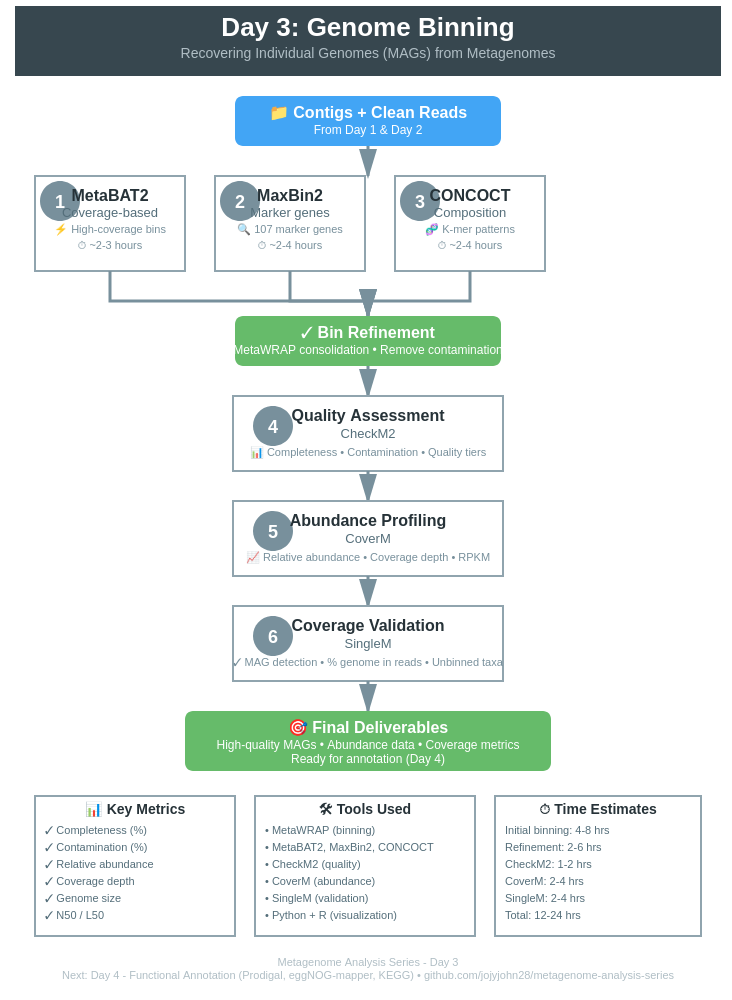
🔄 Binning Workflow
Overview of the Complete Pipeline
Clean FASTQ Files + Contigs (from Day 1 & 2)
                ↓
┌───────────────────────────────────┐
│  MetaWRAP Initial Binning         │
│  (All-in-One Command)             │
│  • Automatic read mapping         │
│  • Coverage calculation           │
│  • MetaBAT2 binning               │
│  • MaxBin2 binning                │
│  • CONCOCT binning                │
│  • CheckM quality assessment      │
└───────────────────────────────────┘
            ↓
┌───────────────────────────────────┐
│  Bin Refinement (MetaWRAP)        │
│  • Consolidate bins               │
│  • Remove contamination           │
│  • Improve completeness           │
│  • Re-validate with CheckM        │
└───────────────────────────────────┘
            ↓
┌───────────────────────────────────┐
│  Quality Assessment (CheckM2)     │
│  • Completeness > 50%             │
│  • Contamination < 10%            │
│  • Quality tiers (HQ/MQ/LQ)       │
└───────────────────────────────────┘
            ↓
┌───────────────────────────────────┐
│  Abundance Profiling (CoverM)     │
│  • Relative abundance             │
│  • Mean coverage depth            │
│  • RPKM / TPM normalization       │
│  • Multi-sample comparison        │
└───────────────────────────────────┘
            ↓
┌───────────────────────────────────┐
│  Coverage Validation (SingleM)    │
│  • MAG detection in samples       │
│  • % genome covered by reads      │
│  • Identify unbinned organisms    │
│  • Strain-level analysis          │
└───────────────────────────────────┘
            ↓
┌───────────────────────────────────┐
│  Bin Quantification (MetaWRAP)    │
│  • Track across time series       │
│  • Core vs variable microbiome    │
│  • Abundance heatmaps             │
└───────────────────────────────────┘
            ↓
High-Quality MAGs + Abundance + Coverage Data
Step 1: Initial Binning with MetaWRAP (All-in-One)
Modern Approach: MetaWRAP can run all three binners (MetaBAT2, MaxBin2, CONCOCT) in a single command!
Why use multiple binners?
- Each algorithm has different strengths
- Combining results improves MAG quality
- Captures more of the community diversity
- MetaWRAP automatically handles coverage calculation
Run MetaWRAP Binning Module
conda activate metawrap

# Run all three binners + CheckM in one command
metawrap binning \
    -o INITIAL_BINNING \
    -t 32 \
    -a contigs.fasta \
    --metabat2 \
    --maxbin2 \
    --concoct \
    clean_reads_R1.fastq \
    clean_reads_R2.fastq \
    -m 1500 \
    --run-checkm
What this does:
- ✅ Maps reads back to contigs automatically
- ✅ Calculates coverage depth
- ✅ Runs MetaBAT2 binning
- ✅ Runs MaxBin2 binning
- ✅ Runs CONCOCT binning
- ✅ Runs CheckM on all bins
- ✅ Generates summary statistics
Parameters explained:
-
-o INITIAL_BINNING: Output directory -
-t 32: Number of threads -
-a contigs.fasta: Assembled contigs from Day 2 -
--metabat2 --maxbin2 --concoct: Enable all three binners -
clean_reads_R1.fastq clean_reads_R2.fastq: Clean reads from Day 1 -
-m 1500: Minimum bin size (1.5 Mb) -
--run-checkm: Run quality assessment immediately
Expected output structure:
INITIAL_BINNING/
├── metabat2_bins/          # MetaBAT2 results
│   ├── bin.1.fa
│   ├── bin.2.fa
│   └── ...
├── maxbin2_bins/           # MaxBin2 results
│   ├── bin.001.fasta
│   ├── bin.002.fasta
│   └── ...
├── concoct_bins/           # CONCOCT results
│   ├── 0.fa
│   ├── 1.fa
│   └── ...
├── metabat2_bins.stats     # CheckM results
├── maxbin2_bins.stats
├── concoct_bins.stats
└── work_files/             # Intermediate files
Time: 4-8 hours depending on data size and number of samples (for me 32 metagenomes took many days in batch to finish the binning)
Algorithm Strengths:
| Binner | Best For | Approach |
|---|---|---|
| MetaBAT2 | High-coverage bins | Coverage + tetranucleotide frequency |
| MaxBin2 | Low-abundance organisms | Marker genes (107 genes) + coverage |
| CONCOCT | Complex communities | Gaussian mixture models on coverage |
Step 2: Bin Refinement with MetaWRAP
Bin refinement consolidates the three binning results to produce the best possible MAGs.
conda activate metawrap

metawrap bin_refinement \
    -o BIN_REFINEMENT \
    -t 32 \
    -A INITIAL_BINNING/metabat2_bins/ \
    -B INITIAL_BINNING/maxbin2_bins/ \
    -C INITIAL_BINNING/concoct_bins/ \
    -c 50 \
    -x 10 \
    -m 1500

# Alternative: Stricter quality thresholds for publication
metawrap bin_refinement \
    -o BIN_REFINEMENT_STRICT \
    -t 32 \
    -A INITIAL_BINNING/metabat2_bins/ \
    -B INITIAL_BINNING/maxbin2_bins/ \
    -C INITIAL_BINNING/concoct_bins/ \
    -c 70 \
    -x 5 \
    -m 1500
Parameters:
-
-o: Output directory -
-t 32: Number of threads -
-A/-B/-C: Paths to the three binning results -
-c 50: Minimum completeness (50%, or 70% for strict) -
-x 10: Maximum contamination (10%, or 5% for strict) -
-m 1500: Minimum bin size (1.5 Mb)
What refinement does:
- Identifies overlapping bins across methods
- Picks best contigs from each method
- Removes contaminating contigs
- Validates with CheckM
- Produces consensus bins
- Creates visualization plots
Expected output:
BIN_REFINEMENT/
├── metawrap_50_10_bins/          # Final refined bins
│   ├── bin.1.fa
│   ├── bin.2.fa
│   └── ...
├── metawrap_50_10_bins.stats     # Quality statistics
├── metawrap_50_10_bins.contigs   # Contig assignments
├── figures/
│   ├── binning_results.png       # Venn diagram
│   └── bin_refinement_stats.png  # Quality metrics
└── work_files/
Step 3: Bin Quality Assessment
# Run CheckM on refined bins
checkm lineage_wf \
    -t 16 \
    -x fa \
    BIN_REFINEMENT/metawrap_50_10_bins/ \
    checkm_output/

# Generate summary table
checkm qa \
    checkm_output/lineage.ms \
    checkm_output/ \
    -o 2 \
    -f checkm_summary.txt \
    --tab_table
Interpreting Results:
| Quality Tier | Completeness | Contamination | Use Case |
|---|---|---|---|
| High-Quality (HQ) | >90% | <5% | Publications, reference genomes |
| Medium-Quality (MQ) | 50-90% | <10% | Most analyses, gene mining |
| Low-Quality (LQ) | <50% | >10% | Exploratory, presence/absence |
Step 4: Bin Quantification (Abundance)
Calculate the abundance of each MAG across your samples:
conda activate metawrap

# Quantify bins across samples
metawrap quant_bins \
    -b BIN_REFINEMENT/metawrap_50_10_bins \
    -o QUANT_BINS \
    -a contigs.fasta \
    clean_reads_*.fastq \
    -t 32

# For multiple samples (time series, spatial)
metawrap quant_bins \
    -b BIN_REFINEMENT/metawrap_50_10_bins \
    -o QUANT_BINS \
    -a contigs.fasta \
    sample1_R*.fastq sample2_R*.fastq sample3_R*.fastq \
    -t 32
What quantification does:
- Maps reads from each sample to refined bins
- Calculates coverage and abundance
- Generates abundance table
- Identifies dominant vs rare community members
Output:
QUANT_BINS/
├── bin_abundance_table.tab        # Abundance matrix
├── bin_abundance_heatmap.png      # Visualization
└── sample_logs/                   # Per-sample mapping logs
Use cases:
- Track MAG abundance across time series
- Compare communities between samples
- Identify core vs variable microbiome members
- Calculate relative abundance
Step 5: MAG Abundance Profiling with CoverM
CoverM provides comprehensive abundance metrics including relative abundance, mean coverage, and RPKM.
Installation
# Install CoverM
conda install -c bioconda coverm

# Verify installation
coverm --version
Calculate MAG Abundance Across Multiple Samples
# Create directory for results
mkdir -p mag_abundance

# Run CoverM genome mode
coverm genome \
    --coupled \
        sample1_R1.fastq.gz sample1_R2.fastq.gz \
        sample2_R1.fastq.gz sample2_R2.fastq.gz \
        sample3_R1.fastq.gz sample3_R2.fastq.gz \
    --genome-fasta-directory BIN_REFINEMENT/metawrap_50_10_bins \
    --genome-fasta-extension fa \
    --output-file mag_abundance/mag_abundance_table.tsv \
    --threads 32 \
    --methods relative_abundance mean trimmed_mean covered_fraction \
    --min-covered-fraction 0.1

# Alternative: If you already have BAM files
coverm genome \
    --bam-files sample1.bam sample2.bam sample3.bam \
    --genome-fasta-directory BIN_REFINEMENT/metawrap_50_10_bins \
    --genome-fasta-extension fa \
    --output-file mag_abundance/mag_abundance_table.tsv \
    --methods relative_abundance mean covered_fraction
CoverM Methods Explained
| Method | Description | When to Use |
|---|---|---|
| relative_abundance | % of total reads mapping to MAG | Community composition |
| mean | Mean coverage depth | Abundance estimation |
| trimmed_mean | Mean after trimming outliers | Robust abundance |
| covered_fraction | % of genome covered by reads | MAG detection confidence |
| rpkm | Reads Per Kilobase per Million | Cross-sample normalization |
| tpm | Transcripts Per Million | RNA-seq abundance |
Analyze CoverM Output
# View abundance table
column -t mag_abundance/mag_abundance_table.tsv | less -S

# Extract relative abundance only
cut -f1,2,5,8,11 mag_abundance/mag_abundance_table.tsv > mag_relative_abundance.tsv
Example output:
Genome              Sample1_RA  Sample2_RA  Sample3_RA  Sample1_Mean  Sample2_Mean
bin.1.fa            15.2        18.4        12.1        45.3          52.1
bin.2.fa            8.7         6.2         9.3         28.4          21.7
bin.3.fa            2.1         3.4         1.8         8.9           12.3
Visualize MAG Abundance
#!/usr/bin/env python3
# visualize_mag_abundance.py

import pandas as pd
import matplotlib.pyplot as plt
import seaborn as sns

# Read CoverM output
df = pd.read_csv('mag_abundance/mag_abundance_table.tsv', sep='\t')

# Extract relative abundance columns (every 3rd column starting from 1)
ra_cols = [col for col in df.columns if 'Relative Abundance' in col]
abundance_df = df[['Genome'] + ra_cols]

# Clean column names
abundance_df.columns = ['MAG'] + [col.split()[0] for col in ra_cols]

# Set MAG as index
abundance_df = abundance_df.set_index('MAG')

# Create heatmap
plt.figure(figsize=(12, 8))
sns.heatmap(abundance_df, annot=True, fmt='.2f', cmap='YlOrRd',
            cbar_kws={'label': 'Relative Abundance (%)'})
plt.title('MAG Relative Abundance Across Samples', fontsize=14, fontweight='bold')
plt.xlabel('Sample', fontsize=12)
plt.ylabel('MAG', fontsize=12)
plt.tight_layout()
plt.savefig('mag_abundance/abundance_heatmap.pdf', dpi=300)
print("✓ Heatmap saved: mag_abundance/abundance_heatmap.pdf")

# Create stacked bar chart
abundance_df.T.plot(kind='bar', stacked=True, figsize=(10, 6),
                     colormap='tab20')
plt.title('MAG Community Composition', fontsize=14, fontweight='bold')
plt.xlabel('Sample', fontsize=12)
plt.ylabel('Relative Abundance (%)', fontsize=12)
plt.legend(title='MAG', bbox_to_anchor=(1.05, 1), loc='upper left')
plt.tight_layout()
plt.savefig('mag_abundance/composition_barplot.pdf', dpi=300)
print("✓ Barplot saved: mag_abundance/composition_barplot.pdf")
Step 6: MAG Detection and Coverage with SingleM
SingleM analyzes what percentage of each MAG is actually represented in your samples using single-copy marker genes.
Why Use SingleM?
- ✅ Strain-level detection: Identify MAG presence even at low abundance
- ✅ Coverage estimation: % of MAG covered by sample reads
- ✅ Completeness check: Validate MAG recovery across samples
- ✅ Compare samples: Track MAG presence/absence across conditions
Installation
# Install SingleM
conda install -c bioconda singlem

# Download database (~2 GB)
singlem data
Run SingleM Analysis
# Create directory for results
mkdir -p singlem_results

# Run SingleM pipe on reads and MAGs
singlem pipe \
    --coupled \
        sample1_R1.fastq.gz sample1_R2.fastq.gz \
    --otu-table singlem_results/sample1_otu_table.tsv \
    --threads 32

# Process all samples
for sample in sample1 sample2 sample3; do
    singlem pipe \
        --coupled ${sample}_R1.fastq.gz ${sample}_R2.fastq.gz \
        --otu-table singlem_results/${sample}_otu_table.tsv \
        --threads 32
done

# Run SingleM on MAGs to get reference profiles
singlem pipe \
    --genome-fasta-files BIN_REFINEMENT/metawrap_50_10_bins/*.fa \
    --otu-table singlem_results/mags_otu_table.tsv \
    --threads 32
Appraise MAG Coverage in Samples
# Compare sample OTUs to MAG OTUs
singlem appraise \
    --metagenome-otu-tables singlem_results/sample*_otu_table.tsv \
    --genome-otu-tables singlem_results/mags_otu_table.tsv \
    --output-binned-otu-table singlem_results/binned_otus.tsv \
    --output-unbinned-otu-table singlem_results/unbinned_otus.tsv

# Calculate MAG recovery percentage
singlem summarise \
    --input-otu-tables singlem_results/sample*_otu_table.tsv \
    --output-otu-table singlem_results/summary_otu_table.tsv

# Detailed appraisal with stats
singlem appraise \
    --metagenome-otu-tables singlem_results/sample*_otu_table.tsv \
    --genome-otu-tables singlem_results/mags_otu_table.tsv \
    --plot singlem_results/appraisal_plot.png \
    --output-found-in-metagenome singlem_results/found_mags.tsv
Interpreting SingleM Results
Binned OTUs (binned_otus.tsv):
MAG        Sample      Gene    Coverage    Marker_count
bin.1.fa   sample1     riboL2  95.2%       14/14
bin.1.fa   sample2     riboL2  78.4%       11/14
bin.2.fa   sample1     riboL2  45.8%       6/14
What this tells you:
- 95.2% coverage: MAG is well-represented in sample1
- 78.4% coverage: MAG present but lower abundance in sample2
- 45.8% coverage: Partial MAG detection (low abundance or incomplete)
Unbinned OTUs (unbinned_otus.tsv):
- Sequences in samples that don’t match any MAG
- Indicates organisms you haven’t recovered
- Useful for identifying missing community members
Visualize SingleM Results
#!/usr/bin/env python3
# visualize_singlem_coverage.py

import pandas as pd
import matplotlib.pyplot as plt
import seaborn as sns

# Read SingleM appraisal results
df = pd.read_csv('singlem_results/found_mags.tsv', sep='\t')

# Create pivot table: MAGs vs Samples
pivot = df.pivot_table(values='Coverage', index='MAG', columns='Sample', aggfunc='mean')

# Plot coverage heatmap
plt.figure(figsize=(10, 8))
sns.heatmap(pivot, annot=True, fmt='.1f', cmap='RdYlGn',
            vmin=0, vmax=100,
            cbar_kws={'label': 'Coverage (%)'})
plt.title('MAG Coverage Across Samples (SingleM)', fontsize=14, fontweight='bold')
plt.xlabel('Sample', fontsize=12)
plt.ylabel('MAG', fontsize=12)
plt.tight_layout()
plt.savefig('singlem_results/mag_coverage_heatmap.pdf', dpi=300)
print("✓ Coverage heatmap saved")

# Calculate summary statistics
print("\n" + "="*60)
print("  MAG DETECTION SUMMARY")
print("="*60)
print(f"\nTotal MAGs analyzed: {len(pivot)}")
print(f"Total samples: {len(pivot.columns)}")
print(f"\nMean coverage: {pivot.mean().mean():.1f}%")
print(f"MAGs with >90% coverage: {(pivot > 90).sum().sum()}")
print(f"MAGs with >50% coverage: {(pivot > 50).sum().sum()}")
print(f"MAGs with <10% coverage: {(pivot < 10).sum().sum()} (likely false positives)")
print("="*60)
Combine CoverM and SingleM Results
Create a comprehensive abundance + coverage table:
#!/usr/bin/env python3
# combine_abundance_coverage.py

import pandas as pd

# Read CoverM abundance
coverm_df = pd.read_csv('mag_abundance/mag_abundance_table.tsv', sep='\t')
ra_cols = [col for col in coverm_df.columns if 'Relative Abundance' in col]
abundance = coverm_df[['Genome'] + ra_cols]

# Read SingleM coverage
singlem_df = pd.read_csv('singlem_results/found_mags.tsv', sep='\t')
coverage_pivot = singlem_df.pivot_table(values='Coverage',
                                         index='MAG',
                                         columns='Sample',
                                         aggfunc='mean')

# Merge
combined = abundance.set_index('Genome').join(coverage_pivot, rsuffix='_coverage')

# Save
combined.to_csv('mag_abundance/combined_abundance_coverage.tsv', sep='\t')

print("✓ Combined table saved: mag_abundance/combined_abundance_coverage.tsv")
print("\nExample output:")
print(combined.head())
Example combined output:
MAG        Sample1_RA  Sample1_Cov  Sample2_RA  Sample2_Cov  Interpretation
bin.1.fa   15.2%       95.2%        18.4%       92.1%        High abundance, well-covered
bin.2.fa   8.7%        78.4%        6.2%        71.3%        Medium abundance, good coverage
bin.3.fa   0.5%        15.2%        0.3%        8.7%         Low abundance, poor coverage
Decision Matrix: Abundance + Coverage
| Relative Abundance | Coverage | Interpretation | Action |
|---|---|---|---|
| High (>5%) | High (>80%) | Abundant, well-recovered | ✓ Use for analysis |
| High (>5%) | Low (<50%) | Abundant but incomplete MAG | Reassemble or refine |
| Low (<1%) | High (>80%) | Rare but complete MAG | ✓ Use with caution |
| Low (<1%) | Low (<50%) | Rare and incomplete | Consider removing |
Summary: Abundance Analysis Workflow
# 1. Basic quantification (MetaWRAP)
metawrap quant_bins ...

# 2. Detailed abundance (CoverM)
coverm genome --methods relative_abundance mean covered_fraction ...

# 3. Coverage validation (SingleM)
singlem pipe ...
singlem appraise ...

# 4. Visualize and combine
python visualize_mag_abundance.py
python visualize_singlem_coverage.py
python combine_abundance_coverage.py
What you learn:
- 📊 Relative abundance: Which MAGs dominate the community
- 📈 Coverage depth: How well each MAG is sampled
- ✅ Detection confidence: % of MAG represented in reads
- 🔍 Missing organisms: Unbinned OTUs indicate gaps in MAG recovery
🤖 SemiBin2 Overview
SemiBin2 is a modern, deep learning-based binner that often outperforms traditional methods.
Why Use SemiBin2?
✅ Deep learning-based - Neural networks learn genomic patterns
✅ Self-supervised - No need for labeled training data
✅ Multi-sample aware - Excellent for time series/spatial data
✅ Fast - GPU acceleration available
✅ High precision - Lower contamination rates
Quick Start
# Single-sample binning
SemiBin single_easy_bin \
    -i contigs.fasta \
    -b contigs.bam \
    -o semibin_output \
    --sequencing-type short_read

# Multi-sample binning (recommended for ≥3 samples)
SemiBin multi_easy_bin \
    -i contigs.fasta \
    -b sample1.bam sample2.bam sample3.bam \
    -o semibin_multi_output \
    --sequencing-type short_read
For Detailed Tutorial
🔗 See my complete SemiBin2 guide →
This covers:
- Installation and setup
- Single vs multi-sample strategies
- GPU acceleration
- Parameter optimization
- Integration with MetaWRAP
- Benchmarking against other binners
🔍 Quality Assessment with CheckM2
CheckM2 is the modern successor to CheckM - faster, more accurate, and easier to use.
Why CheckM2 > CheckM?
| Feature | CheckM2 | CheckM (old) |
|---|---|---|
| Speed | 13x faster | Slow |
| Database | 21,000 genomes | 5,000 genomes |
| Memory | Low | High |
| Accuracy | Higher | Good |
| Installation | Easy | Complex |
Installation & Setup
conda activate metawrap

# Install CheckM2
conda install -c bioconda checkm2

# Download database (~3.5 GB, one-time)
checkm2 database --download --path ~/checkm2_db/

# Verify installation
checkm2 --version
Running CheckM2
# Assess all refined bins
checkm2 predict \
    --threads 16 \
    --input BIN_REFINEMENT/metawrap_50_10_bins \
    --output-directory checkm2_output \
    -x fa

# Generate quality report
checkm2 quality_report \
    --tsv_file checkm2_output/quality_report.tsv
Interpreting Output
Key Metrics:
- Completeness - % of expected marker genes found
-
90% = Excellent
- 70-90% = Good
- 50-70% = Fair
- <50% = Incomplete
-
- Contamination - % of duplicated marker genes
- <5% = Excellent
- 5-10% = Acceptable
-
10% = Needs refinement
- Strain Heterogeneity - Mixed strains indicator
- Low = Single strain
- High = Multiple strains mixed
Example output:
Name      Completeness  Contamination  Strain_heterogeneity
bin.1     95.2%        2.1%           0.0%          # HQ MAG
bin.2     87.3%        8.5%           10.2%         # MQ MAG
bin.3     45.8%        15.3%          25.6%         # LQ MAG - discard
Quality Filtering
# Keep only high/medium quality MAGs
python << 'EOF'
import pandas as pd

# Read CheckM2 output
df = pd.read_csv('checkm2_output/quality_report.tsv', sep='\t')

# Define quality thresholds
hq = df[(df['Completeness'] > 90) & (df['Contamination'] < 5)]
mq = df[(df['Completeness'] > 50) & (df['Contamination'] < 10)]

print(f"High-quality MAGs: {len(hq)}")
print(f"Medium-quality MAGs: {len(mq)}")

# Save filtered list
mq.to_csv('quality_mags.csv', index=False)
EOF
📊 Visualizing Results
Create Bin Quality Plot
#!/usr/bin/env python3
# plot_bin_quality.py

import pandas as pd
import matplotlib.pyplot as plt
import seaborn as sns

# Read CheckM2 output
df = pd.read_csv('checkm2_output/quality_report.tsv', sep='\t')

# Create scatter plot
plt.figure(figsize=(10, 8))
scatter = plt.scatter(df['Contamination'], df['Completeness'],
                     s=100, alpha=0.6, c=df['Completeness']-df['Contamination'],
                     cmap='RdYlGn')

# Add quality thresholds
plt.axhline(y=90, color='green', linestyle='--', label='HQ threshold (90%)')
plt.axhline(y=50, color='orange', linestyle='--', label='MQ threshold (50%)')
plt.axvline(x=5, color='green', linestyle='--', label='HQ contamination (5%)')
plt.axvline(x=10, color='orange', linestyle='--', label='MQ contamination (10%)')

plt.xlabel('Contamination (%)', fontsize=12)
plt.ylabel('Completeness (%)', fontsize=12)
plt.title('MAG Quality Assessment', fontsize=14, fontweight='bold')
plt.colorbar(scatter, label='Quality Score (Comp - Cont)')
plt.legend()
plt.grid(alpha=0.3)
plt.tight_layout()
plt.savefig('mag_quality.pdf', dpi=300)
plt.savefig('mag_quality.png', dpi=300)
print("✓ Plot saved: mag_quality.pdf/png")
Generate Summary Report
python << 'EOF'
import pandas as pd
from collections import Counter

# Read data
checkm = pd.read_csv('checkm2_output/quality_report.tsv', sep='\t')
gtdbtk = pd.read_csv('gtdbtk_output/gtdbtk.bac120.summary.tsv', sep='\t')

# Quality summary
hq = len(checkm[(checkm['Completeness']>90) & (checkm['Contamination']<5)])
mq = len(checkm[(checkm['Completeness']>50) & (checkm['Contamination']<10) &
                ~((checkm['Completeness']>90) & (checkm['Contamination']<5))])
lq = len(checkm) - hq - mq

print("="*60)
print("  MAG Recovery Summary")
print("="*60)
print(f"Total bins recovered: {len(checkm)}")
print(f"  High-quality (HQ):    {hq} ({hq/len(checkm)*100:.1f}%)")
print(f"  Medium-quality (MQ):  {mq} ({mq/len(checkm)*100:.1f}%)")
print(f"  Low-quality (LQ):     {lq} ({lq/len(checkm)*100:.1f}%)")
print()

# Taxonomy summary
phyla = [tax.split(';')[1] for tax in gtdbtk['classification']]
phyla_counts = Counter(phyla)

print("Top 5 Phyla:")
for phylum, count in phyla_counts.most_common(5):
    print(f"  {phylum}: {count} MAGs")
print()

# Size statistics
print("Genome Size Statistics:")
print(f"  Mean: {checkm['Genome_size'].mean()/1e6:.2f} Mb")
print(f"  Median: {checkm['Genome_size'].median()/1e6:.2f} Mb")
print(f"  Range: {checkm['Genome_size'].min()/1e6:.2f} - {checkm['Genome_size'].max()/1e6:.2f} Mb")
print("="*60)
EOF
💡 Best Practices
Before Binning
- ✅ Good assembly quality (N50 > 5kb recommended)
- ✅ Sufficient coverage (>10x mean coverage minimum)
- ✅ Multiple samples (if available) improve binning
- ✅ Long contigs (>2500 bp) bin better
- ✅ Clean data from Day 1 QC
During Binning
- ✅ Use multiple binners (3+ recommended)
- ✅ Refine bins with MetaWRAP or DAS Tool
- ✅ Document parameters for reproducibility
- ✅ Monitor resources (disk space, memory)
- ✅ Save intermediate files until verified
After Binning
- ✅ Quality check ALL bins with CheckM2
- ✅ Filter by quality (keep MQ+ for most analyses)
- ✅ Classify taxonomically with GTDB-Tk
- ✅ Dereplicate if many similar MAGs
- ✅ Backup MAGs - they’re valuable!
Quality Thresholds by Use Case
| Use Case | Min Completeness | Max Contamination |
|---|---|---|
| Reference genome | 95% | 2% |
| Publication | 90% | 5% |
| Gene mining | 70% | 10% |
| Metabolic analysis | 50% | 10% |
| Presence/absence | 50% | 15% |
🔧 Troubleshooting
Problem: Few or No Bins Recovered
Possible causes:
- Low sequencing depth
- Poor assembly quality
- High community complexity
- Incorrect coverage calculation
Solutions:
- Check assembly N50 (should be >1kb)
- Verify coverage file is correct
-
Adjust binning parameters:
# Lower minimum bin size metabat2 -m 1000 # instead of 1500 # Lower minimum contig length --minContig 1500 # instead of 2500 - Try SemiBin2 (often better for complex samples)
Problem: High Contamination in Bins
Solutions:
-
Stricter refinement:
metawrap bin_refinement -c 70 -x 5 # More stringent -
Manual curation:
# Use RefineM for interactive refinement conda install -c bioconda refinem refinem scaffold_stats -c 70 -x 5 bins/ bins/ -
Re-bin with different parameters
Problem: MetaWRAP Refinement Fails
Common issues:
Issue 1: Prokka fails
# Verify Prokka environment
conda activate prokka
prokka --version

# Re-install if needed
conda remove prokka
conda install -c bioconda prokka
Issue 2: CheckM database missing
# Download CheckM database
checkm data setRoot ~/checkm_db/
Issue 3: Memory issues
# Reduce threads
metawrap bin_refinement -t 8  # instead of 32

# Or use checkm_lite mode (faster, less memory)
metawrap bin_refinement --quick
Problem: CheckM2 Fails
Solutions:
# Re-download database
rm -rf ~/checkm2_db/
checkm2 database --download --path ~/checkm2_db/

# Verify database integrity
checkm2 testrun

# Check available memory
free -h  # Need at least 16GB

# Reduce parallel jobs if memory limited
checkm2 predict --threads 8  # instead of 16
📈 Expected Results
Typical Recovery Rates
| Sample Type | Expected HQ MAGs | Expected MQ MAGs |
|---|---|---|
| Soil | 5-20 | 20-50 |
| Human gut | 10-40 | 30-80 |
| Marine | 5-15 | 15-40 |
| Wastewater | 10-30 | 30-70 |
Factors affecting recovery:
- Community complexity (α-diversity)
- Sequencing depth (>20M reads = better)
- Assembly quality (N50 >5kb = better)
- Number of samples (more = better for SemiBin2)
Benchmark Comparison
On a mock community (known composition):
| Binner | Precision | Recall | F1-Score |
|---|---|---|---|
| SemiBin2 | 96% | 94% | 95% |
| MetaWRAP Refined | 94% | 91% | 92.5% |
| MetaBAT2 | 90% | 88% | 89% |
| MaxBin2 | 88% | 89% | 88.5% |
| CONCOCT | 85% | 86% | 85.5% |
Higher is better; refinement improves both metrics
✅ Success Checklist
Before moving to Day 4:
- Multiple binners run successfully (3+ recommended)
- Bins refined with MetaWRAP or DAS Tool
- CheckM2 quality assessment completed
- At least 5-10 MQ+ MAGs recovered
- Quality plots generated
- MAGs organized in final directory
📚 Key Papers & Resources
Essential Reading
- Binning Methods:
- Kang et al. (2019) - MetaBAT2: PeerJ
- Wu et al. (2016) - MaxBin2: Bioinformatics
- Alneberg et al. (2014) - CONCOCT: Nature Methods
- Pan et al. (2022) - SemiBin2: Nature Communications
- Quality Assessment:
- Chklovski et al. (2023) - CheckM2: Nature Methods
- Parks et al. (2015) - CheckM: Genome Research
- Refinement:
- Uritskiy et al. (2018) - MetaWRAP: Microbiome
- Sieber et al. (2018) - DAS Tool: Nature Microbiology
Helpful Links
➡️ What’s Next?
Congratulations! You’ve recovered individual genomes from your metagenome!
Day 4: Genome Dereplication & Taxonomic Classification (Coming Soon)
- Dereplicate - Remove redundant genomes, keep best representatives
- Classify - Assign accurate taxonomic names using GTDB
- Visualize - Create beautiful phylogenetic trees
- Curate - Select species representatives for downstream analysis
💬 Feedback
Found this helpful? Have suggestions?
Repo for today’s code and other details
Last updated: February 2025_