Day 2: Metagenome Assembly - Reconstructing Genomes from Short Reads
Day 2: Metagenome Assembly - Reconstructing Genomes from Short Reads
Table of Contents
- Introduction
- Assembly Fundamentals
- Assembler Comparison
- metaSPAdes Assembly
- MEGAHIT Assembly
- Other Assembly Tools
- Long-Read Assembly (ONT/PacBio)
- Assembly Quality Assessment
- Parameter Optimization
- Multi-Language Analysis
- Desktop Tutorial
- Best Practices
- Troubleshooting
Introduction
Welcome to Day 2 of our metagenome analysis series! After quality control and taxonomic profiling in Day 1, we now tackle one of the most computationally intensive and critical steps: de novo metagenome assembly.
What is Metagenome Assembly?
Assembly is the process of reconstructing longer DNA sequences (contigs and scaffolds) from millions of short sequencing reads. Unlike single-genome assembly, metagenomic assembly is particularly challenging because:
- Multiple genomes present simultaneously
- Varying abundance (high to extremely low)
- Strain variation within species
- Repetitive sequences shared across organisms
- Uneven sequencing coverage
Why Assembly Matters
Assembly is crucial for:
- 📊 Recovering complete or near-complete genomes (MAGs)
- 🧬 Identifying novel genes and biosynthetic gene clusters
- 🔬 Enabling functional annotation beyond marker genes
- 🌐 Understanding genomic context
- 📈 Improving resolution of community structure
What You’ll Learn Today
By the end of this tutorial, you’ll be able to:
- ✅ Assemble metagenomes using multiple assemblers
- ✅ Understand assembly parameters and optimization
- ✅ Assess assembly quality with MetaQUAST
- ✅ Compare different assembly strategies
- ✅ Use Python and R for assembly analysis
- ✅ Run assemblies on desktop (with limited resources)
- ✅ Handle both short-read and long-read data
Assembly Fundamentals
The De Bruijn Graph Approach
Modern metagenomic assemblers use de Bruijn graphs to construct contigs:
- K-mer decomposition: Reads are broken into overlapping k-mers
- Graph construction: K-mers become nodes, overlaps become edges
- Path finding: Contigs are paths through the graph
- Graph simplification: Remove bubbles, tips, and low-coverage paths
Key Concepts
Contig: A contiguous assembled sequence with no gaps
Scaffold: Multiple contigs connected by gap information (paired-end/mate-pair reads)
N50: The contig length at which 50% of the assembly is in contigs of this size or larger (higher is better)
Coverage: Average number of reads covering each base position
k-mer size: Length of subsequences used in assembly (critical parameter!)
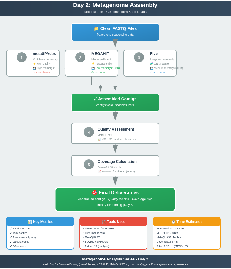
Assembler Comparison
metaSPAdes vs MEGAHIT vs Others
| Feature | metaSPAdes | MEGAHIT | IDBA-UD | Flye (Long-read) |
|---|---|---|---|---|
| Algorithm | Multi-k-mer SPAdes | Succinct de Bruijn | Multi-k-mer IDBA | Repeat graph |
| Memory Usage | High (64-256 GB) | Low (16-64 GB) | Medium (32-128 GB) | Medium (32-128 GB) |
| Speed | Slow (hours-days) | Fast (30min-hours) | Medium (hours) | Medium (hours) |
| Contig Quality | Excellent | Very Good | Good | Excellent |
| N50 | Highest | High | Medium | Very High |
| Best For | High-quality assemblies | Large datasets, limited RAM | Uneven coverage | Long reads (ONT/PacBio) |
| Max k-mer | 127 (default) | 255 | 124 | N/A (overlap-based) |
| Error Correction | Built-in BayesHammer | Basic | Moderate | Consensus-based |
| Read Type | Illumina | Illumina | Illumina | ONT/PacBio |
| Hybrid Mode | Yes (trusted contigs) | No | Limited | Yes (with Illumina polishing) |
| Typical RAM | 100-200 GB | 30-60 GB | 60-100 GB | 50-120 GB |
| Typical Time | 12-48 hours | 2-8 hours | 6-24 hours | 4-16 hours |
| Citation | Nurk et al. 2017 | Li et al. 2015 | Peng et al. 2012 | Kolmogorov et al. 2019 |
When to Use Which Assembler?
Use metaSPAdes when:
- ✅ You need the highest quality assembly
- ✅ You have access to HPC with ample RAM (128GB+)
- ✅ Assembly time is not critical
- ✅ You’re working with complex metagenomes
- ✅ You want the best N50 and fewer misassemblies
Use MEGAHIT when:
- ✅ You have limited computational resources
- ✅ You need fast results (rapid prototyping)
- ✅ You’re assembling very large datasets (100GB+)
- ✅ You’re running on a desktop or laptop
- ✅ Memory is the limiting factor
Use IDBA-UD when:
- ✅ You have highly uneven coverage
- ✅ You want a middle ground between metaSPAdes and MEGAHIT
- ✅ You have specific experience with IDBA
Use Flye when:
- ✅ You have long-read data (ONT/PacBio)
- ✅ You want to resolve repetitive regions
- ✅ You’re doing hybrid assembly (long + short reads)
Recommendation
For this tutorial, we’ll focus on metaSPAdes (gold standard) and MEGAHIT (practical alternative). We’ll also cover Flye basics for long-read enthusiasts.
Which Assembler Should I Use? (Quick Decision Guide)
Use this decision tree to quickly choose the right assembler for your situation:
START
  │
  ├─ What type of reads do you have?
  │   ├─ Illumina short reads → Continue below
  │   ├─ ONT/PacBio long reads → Use Flye (--meta)
  │   └─ Both (hybrid) → Use Flye + Pilon polishing
  │
  ├─ How much RAM do you have?
  │   ├─ ≤16 GB (laptop/desktop) → Use MEGAHIT
  │   ├─ 32-64 GB (workstation) → Use MEGAHIT or IDBA-UD
  │   └─ ≥128 GB (HPC) → Use metaSPAdes
  │
  ├─ What's your priority?
  │   ├─ Highest quality assembly → Use metaSPAdes
  │   ├─ Fastest results → Use MEGAHIT
  │   └─ Uneven coverage → Use IDBA-UD
  │
  └─ Special cases:
      ├─ Very large dataset (>100 GB) → Use MEGAHIT
      ├─ Extremely uneven coverage → Use IDBA-UD
      └─ Novel/complex metagenome → Use metaSPAdes
Quick Reference Table
| Your Situation | Recommended Assembler | Alternative |
|---|---|---|
| 💻 Laptop (8-16GB RAM) | MEGAHIT | Subsample + metaSPAdes |
| 🖥️ Desktop (32-64GB RAM) | MEGAHIT or IDBA-UD | metaSPAdes (small samples) |
| 🏢 HPC (128GB+ RAM) | metaSPAdes | MEGAHIT (for speed) |
| 📊 Uneven coverage | IDBA-UD | metaSPAdes |
| 🧬 Long reads (ONT) | Flye –meta | metaFlye |
| 🧬 Long reads (PacBio) | Flye –pacbio-hifi | Hifiasm-meta |
| 🔬 Hybrid (long + short) | Flye + Pilon | metaSPAdes + long-read scaffolding |
| ⚡ Need speed | MEGAHIT | Skip assembly, use reads directly |
| 🎯 Need quality | metaSPAdes | Multiple assemblers + comparison |
Real-World Examples
Scenario 1: PhD Student with Laptop
- RAM: 16 GB
- Sample: Human gut metagenome
- Solution: Subsample to 2M reads → MEGAHIT → 2-3 hours
Scenario 2: Research Lab with HPC
- RAM: 256 GB
- Sample: Soil metagenome (complex)
- Solution: metaSPAdes with default parameters → 24-36 hours
Scenario 3: Clinical Lab, Time-Critical
- RAM: 64 GB
- Sample: Patient sample
- Solution: MEGAHIT (meta-sensitive preset) → 3-4 hours
Scenario 4: Long-Read Sequencing Project
- Data: ONT reads (N50=15kb)
- Solution: Flye –nano-hq –meta → Polish with Medaka → 6-8 hours
metaSPAdes Assembly
metaSPAdes is part of the SPAdes assembler family, specifically designed for metagenomic data.
Installation
# Using conda (recommended)
conda install -c bioconda spades

# Or download binary
wget http://cab.spbu.ru/files/release3.15.5/SPAdes-3.15.5-Linux.tar.gz
tar -xzf SPAdes-3.15.5-Linux.tar.gz
export PATH=$PATH:/path/to/SPAdes-3.15.5-Linux/bin
Basic Usage
# Single sample, paired-end
metaspades.py \
    -1 clean_R1.fastq.gz \
    -2 clean_R2.fastq.gz \
    -o metaspades_output \
    -t 32 \
    -m 200

# Options explained:
# -1/-2    : Paired-end input files
# -o       : Output directory
# -t       : Number of threads
# -m       : Memory limit in GB
Important Parameters
K-mer sizes (-k):
# Default: automatic selection (21,33,55,77,99,127)
metaspades.py -k 21,33,55,77,99,127 ...

# For low-complexity samples:
metaspades.py -k 21,33,55,77 ...

# For high-quality, deep sequencing:
metaspades.py -k 33,55,77,99,127 ...
Coverage cutoff (--cov-cutoff):
# Auto (recommended):
--cov-cutoff auto

# Manual (if you know your coverage):
--cov-cutoff 5  # Remove contigs with <5x coverage
Additional options:
# Continue from checkpoint (if interrupted)
metaspades.py --continue -o metaspades_output

# Use only contigs >500bp
# (controlled post-assembly, not during)
Understanding metaSPAdes Output
metaspades_output/
├── assembly_graph.fastg          # Assembly graph
├── assembly_graph_with_scaffolds.gfa  # Scaffold graph
├── before_rr.fasta              # Before repeat resolution
├── contigs.fasta                # Final contigs
├── scaffolds.fasta              # Final scaffolds
├── contigs.paths                # Contig paths
├── scaffolds.paths              # Scaffold paths
├── K21/                         # K-mer 21 assembly
├── K33/                         # K-mer 33 assembly
├── ...
├── params.txt                   # Parameters used
├── spades.log                   # Assembly log
└── warnings.log                 # Warnings
Key files:
- contigs.fasta: Use for binning and annotation
- scaffolds.fasta: Use if you need scaffold information
- spades.log: Check for errors and statistics
Contigs vs Scaffolds: Which Should I Use?
IMPORTANT: This is a common source of confusion for beginners!
✅ Use contigs.fasta for:
- Genome binning (MetaBAT2, MaxBin2, CONCOCT, SemiBin)
- Coverage calculation (essential for Day 3)
- Functional annotation (Prokka, DRAM)
- Gene prediction (Prodigal)
- Most downstream analyses
⚠️ Use scaffolds.fasta ONLY if:
- You need scaffold-level information for specific analyses
- You understand how to handle gaps (N’s in sequences)
- You’re doing structural genomic analysis
- You’re specifically asked to use scaffolds by a tool
Why contigs for binning?
Scaffolds contain gaps (represented by N’s) where paired-end information suggests two contigs are connected, but the exact sequence is unknown. These gaps can:
- Interfere with coverage calculation
- Cause issues with gene prediction
- Create artificial breaks in binning algorithms
Example:
Contig:   ATCGATCGATCG (actual sequence, 100% certain)
Scaffold: ATCGATCG[NNNNNNNN]ATCGATCG (contig + gap + contig)
Rule of thumb: If you’re not sure, use contigs.fasta. You can always generate scaffolds later if needed.
Example Output Statistics
Contigs:
  Total: 125,842
  >= 500 bp: 45,231
  >= 1000 bp: 28,567
  >= 5000 bp: 8,234

Total length: 345,678,901 bp
N50: 2,847 bp
N75: 1,234 bp
Longest contig: 234,567 bp
MEGAHIT Assembly
MEGAHIT is designed for efficiency, using a succinct de Bruijn graph.
Installation
# Using conda
conda install -c bioconda megahit

# Or from source
git clone https://github.com/voutcn/megahit.git
cd megahit
make
Basic Usage
# Single sample
megahit \
    -1 clean_R1.fastq.gz \
    -2 clean_R2.fastq.gz \
    -o megahit_output \
    -t 32 \
    -m 0.9

# Options explained:
# -m 0.9   : Use 90% of available memory
# -t       : Number of threads
Important Parameters
K-mer range:
# Default: 21,29,39,59,79,99,119,141
megahit --k-min 21 --k-max 141 --k-step 20 ...

# For low-complexity:
megahit --k-min 21 --k-max 99 --k-step 20 ...

# For high-quality data:
megahit --k-min 27 --k-max 127 --k-step 20 ...
Presets:
# For metagenomic data (default)
megahit --presets meta-sensitive ...

# For large and complex metagenomes
megahit --presets meta-large ...
Minimum contig length:
# Filter short contigs (default: 200)
megahit --min-contig-len 500 ...
MEGAHIT Output
megahit_output/
├── final.contigs.fa             # Final assembly
├── intermediate_contigs/        # Intermediate k-mer assemblies
├── log                          # Assembly log
└── options.json                 # Parameters used
Memory Efficiency Tips
# Use memory efficiently
megahit -m 0.8 ...  # Use 80% of RAM

# For very large datasets, use:
megahit --mem-flag 2 ...  # Reduce memory at cost of speed
Other Assembly Tools
IDBA-UD (Iterative de Bruijn graph Assembler for Uneven Depth)
Strengths:
- Handles uneven coverage well
- Good for samples with extreme abundance variation
Installation:
conda install -c bioconda idba
Usage:
# IDBA requires fasta input
fq2fa --merge clean_R1.fastq.gz clean_R2.fastq.gz reads.fasta

# Run assembly
idba_ud -r reads.fasta -o idba_output --num_threads 32 --mink 20 --maxk 120 --step 20
Other Notable Assemblers
Ray Meta: Distributed assembler (for clusters) metaVelvet: Early metagenomic assembler (deprecated) OPERA-MS: Hybrid assembler using reference genomes SOAPdenovo2: Large-scale assembler (memory-intensive)
Long-Read Assembly (ONT/PacBio)
Why Long Reads?
Oxford Nanopore (ONT) and PacBio provide reads of 10kb-100kb+, enabling:
- ✅ Better resolution of repetitive regions
- ✅ Complete genomes with fewer contigs
- ✅ Improved scaffold quality
- ✅ Structural variant detection
Flye for Metagenomic Long Reads
Installation:
conda install -c bioconda flye
Basic Usage:
# ONT raw reads
flye --nano-raw ont_reads.fastq.gz \
     --out-dir flye_output \
     --threads 32 \
     --meta

# ONT high-quality reads (Guppy5+)
flye --nano-hq ont_reads.fastq.gz \
     --out-dir flye_output \
     --threads 32 \
     --meta

# PacBio HiFi reads
flye --pacbio-hifi hifi_reads.fastq.gz \
     --out-dir flye_output \
     --threads 32 \
     --meta
Important: Always use the --meta flag for metagenomic data!
metaFlye
metaFlye is specifically designed for metagenomic long reads:
# Same as flye with --meta flag
flye --nano-raw reads.fastq.gz --meta --out-dir metaflye_output --threads 32
Hybrid Assembly (Long + Short Reads)
Strategy 1: Long-read assembly + short-read polishing
# 1. Assemble with Flye
flye --nano-raw ont_reads.fastq.gz --meta -o flye_output -t 32

# 2. Polish with Illumina reads using Pilon
bwa index flye_output/assembly.fasta
bwa mem -t 32 flye_output/assembly.fasta illumina_R1.fastq.gz illumina_R2.fastq.gz | \
    samtools sort -o aligned.bam
samtools index aligned.bam

pilon --genome flye_output/assembly.fasta \
      --frags aligned.bam \
      --output polished \
      --threads 32
Strategy 2: Short-read assembly + long-read scaffolding
# 1. Assemble with metaSPAdes
metaspades.py -1 R1.fastq.gz -2 R2.fastq.gz -o spades_output -t 32

# 2. Scaffold with long reads using npScarf
npScarf -s spades_output/scaffolds.fasta \
        -l ont_reads.fastq.gz \
        -o scaffolded.fasta \
        -t 32
Recommendations for Long-Read Assembly
| Data Type | Recommended Assembler | Polishing |
|---|---|---|
| ONT (raw, <90% accuracy) | Flye | Racon + Medaka |
| ONT (HQ, >95% accuracy) | Flye (–nano-hq) | Medaka or Pilon |
| PacBio HiFi | Flye or Hifiasm-meta | Usually not needed |
| Hybrid (ONT + Illumina) | Flye + Pilon | Pilon (Illumina) |
| Hybrid (PacBio + Illumina) | Flye + Pilon | Pilon (Illumina) |
Assembly Quality Assessment
MetaQUAST: The Standard for Assembly Evaluation
MetaQUAST (Quality Assessment Tool for Metagenome Assemblies) provides comprehensive quality metrics.
Installation:
conda install -c bioconda quast
Basic Usage:
# Single assembly
metaquast.py contigs.fasta -o metaquast_output -t 32

# Multiple assemblies (comparison)
metaquast.py \
    metaspades_contigs.fasta \
    megahit_contigs.fasta \
    idba_contigs.fasta \
    -o metaquast_comparison \
    -t 32 \
    --labels metaSPAdes,MEGAHIT,IDBA-UD

# With reference genomes (if available)
metaquast.py contigs.fasta \
    -r reference_genomes/*.fasta \
    -o metaquast_with_ref \
    -t 32
Understanding MetaQUAST Output
metaquast_output/
├── report.html              # Interactive HTML report
├── report.pdf               # PDF report
├── report.txt               # Text summary
├── report.tsv               # Tab-separated values
├── contigs_reports/         # Per-contig statistics
├── basic_stats/             # Basic statistics
└── icarus.html             # Contig browser
Key Metrics Explained
Basic Statistics:
- # contigs: Total number of contigs
- Largest contig: Length of longest contig
- Total length: Sum of all contig lengths
- N50: Contig length at 50% of assembly
- L50: Number of contigs comprising 50% of assembly
Example:
# contigs (>= 0 bp):       125,842
# contigs (>= 1000 bp):     28,567
# contigs (>= 5000 bp):      8,234
# contigs (>= 10000 bp):     3,456
# contigs (>= 25000 bp):       892
# contigs (>= 50000 bp):       234

Total length (>= 0 bp):      345,678,901
Total length (>= 1000 bp):   298,456,123
Total length (>= 5000 bp):   245,123,456
Total length (>= 10000 bp):  198,765,432
Total length (>= 25000 bp):  145,234,567
Total length (>= 50000 bp):   89,012,345

Largest contig:              234,567
N50:                          2,847
N75:                          1,234
L50:                         32,456
L75:                         78,901

GC (%):                       52.34
What Makes a Good Assembly?
| Metric | Poor | Acceptable | Good | Excellent |
|---|---|---|---|---|
| N50 | <1 kb | 1-5 kb | 5-20 kb | >20 kb |
| # contigs (>1kb) | >100k | 50-100k | 10-50k | <10k |
| Largest contig | <10 kb | 10-50 kb | 50-200 kb | >200 kb |
| Total length | Variable | Variable | Variable | Variable |
| L50 | >50k | 20-50k | 5-20k | <5k |
| Misassemblies* | >1000 | 100-1000 | 10-100 | <10 |
*When reference genomes available
Parameter Optimization
K-mer Size Selection
General guidelines:
- Shorter k-mers (21-55): Better for low coverage, high error rate
- Longer k-mers (77-127): Better for high coverage, low error rate
- Multiple k-mers: Best approach (used by metaSPAdes, MEGAHIT)
Empirical testing:
# Test different k-mer ranges
for KMAX in 99 127 141; do
    megahit -1 R1.fq.gz -2 R2.fq.gz \
            --k-max ${KMAX} \
            -o megahit_k${KMAX} \
            -t 32
done

# Compare with MetaQUAST
metaquast.py megahit_k*/final.contigs.fa \
    -o kmer_comparison \
    --labels k99,k127,k141
Coverage Cutoff Optimization
# metaSPAdes with different cutoffs
for COV in auto 3 5 10; do
    metaspades.py -1 R1.fq.gz -2 R2.fq.gz \
        --cov-cutoff ${COV} \
        -o spades_cov${COV} \
        -t 32 -m 200
done
Assembly Strategy Comparison
Test multiple assemblers and parameters:
#!/bin/bash
# assembly_comparison.sh

# metaSPAdes default
metaspades.py -1 R1.fq.gz -2 R2.fq.gz -o spades_default -t 32 -m 200

# metaSPAdes optimized
metaspades.py -1 R1.fq.gz -2 R2.fq.gz -o spades_opt \
    -k 33,55,77,99,127 --cov-cutoff 5 -t 32 -m 200

# MEGAHIT default
megahit -1 R1.fq.gz -2 R2.fq.gz -o megahit_default -t 32

# MEGAHIT meta-large
megahit -1 R1.fq.gz -2 R2.fq.gz -o megahit_large \
    --presets meta-large -t 32

# Compare all
metaquast.py \
    spades_default/contigs.fasta \
    spades_opt/contigs.fasta \
    megahit_default/final.contigs.fa \
    megahit_large/final.contigs.fa \
    -o assembly_comparison \
    --labels SPAdes_def,SPAdes_opt,MEGAHIT_def,MEGAHIT_large \
    -t 32
Multi-Language Analysis
Python Scripts for Assembly Analysis
See: scripts/01_parse_metaquast.py
R Scripts for Visualization
See: scripts/02_assembly_visualization.R
Bash Scripts for Automation
All batch processing scripts available in: scripts/
Desktop Tutorial
Running Assembly on Your Laptop
💻 Desktop Resources: You can absolutely learn metagenome assembly on your personal computer! We provide optimized workflows for systems with 8-16GB RAM.
For complete desktop tutorial with step-by-step instructions, see: RUNNING_ON_LAPTOP.md
Quick Desktop Guide:
- Subsample your data to 500K-1M read pairs
- Use MEGAHIT (memory-efficient)
- Limit threads to n-2 cores
- Monitor RAM usage with
htop - Expect 2-4 hours for small datasets
Preparing for Day 3: Coverage Calculation
Before moving to genome binning (Day 3), you’ll need to calculate contig coverage. This is essential for all binning algorithms!
Why Coverage Matters for Binning
Binning algorithms use coverage information to:
- Group contigs from the same organism (similar coverage patterns)
- Distinguish high-abundance from low-abundance organisms
- Improve bin quality and completeness
Quick Coverage Calculation
# 1. Build Bowtie2 index from your assembly
bowtie2-build contigs.fasta contigs_index

# 2. Map cleaned reads back to contigs
bowtie2 -x contigs_index \
        -1 clean_R1.fastq.gz \
        -2 clean_R2.fastq.gz \
        -p 32 \
        --no-unal | \
    samtools view -bS - | \
    samtools sort -o contigs.bam -

# 3. Index the BAM file
samtools index contigs.bam

# 4. Calculate coverage statistics
samtools depth contigs.bam > contigs_depth.txt

# Or calculate per-contig coverage
samtools coverage contigs.bam > contigs_coverage.txt
Understanding the Output
contigs_depth.txt (per-base depth):
contig1    1    45
contig1    2    47
contig1    3    48
...
contigs_coverage.txt (per-contig summary):
#rname          startpos  endpos  numreads  covbases  coverage  meandepth  meanbaseq  meanmapq
contig1         1         5432    15234     5432      100       45.3       37.2       60
contig2         1         12456   8765      12456     100       38.7       36.8       60
Alternative: Using MetaBAT’s jgi_summarize_bam_contig_depths
This is the preferred method for binning:
# Map reads (as above)
bowtie2-build contigs.fasta contigs_index
bowtie2 -x contigs_index -1 R1.fastq.gz -2 R2.fastq.gz -p 32 | \
    samtools sort -o contigs.bam -
samtools index contigs.bam

# Calculate coverage for MetaBAT
jgi_summarize_bam_contig_depths --outputDepth depth.txt contigs.bam
Output (depth.txt):
contigName      contigLen   totalAvgDepth   sample1.bam   sample1.bam-var
contig1         5432        45.3            45.3          2.1
contig2         12456       38.7            38.7          1.8
For Multiple Samples
If you have multiple samples (essential for co-assembly binning):
# Map each sample
for sample in sample1 sample2 sample3; do
    bowtie2 -x contigs_index \
            -1 ${sample}_R1.fastq.gz \
            -2 ${sample}_R2.fastq.gz \
            -p 32 | \
        samtools sort -o ${sample}.bam -
    samtools index ${sample}.bam
done

# Calculate coverage across all samples
jgi_summarize_bam_contig_depths --outputDepth depth_all_samples.txt *.bam
Time Estimates
| Step | Small Sample (5M pairs) | Medium Sample (20M pairs) | Large Sample (50M pairs) |
|---|---|---|---|
| Index building | 2-5 min | 5-10 min | 10-20 min |
| Read mapping | 30-60 min | 2-4 hours | 6-12 hours |
| BAM sorting | 5-10 min | 20-40 min | 1-2 hours |
| Coverage calc | 2-5 min | 10-20 min | 30-60 min |
| Total | ~1 hour | ~3-5 hours | ~8-15 hours |
Checkpoint: Files Needed for Day 3
Before starting Day 3, ensure you have:
- ✅
contigs.fasta- Your assembled contigs - ✅
contigs.bam- Mapped reads (sorted and indexed) - ✅
contigs.bam.bai- BAM index file - ✅
depth.txt- Coverage information (from jgi_summarize)
We’ll use these files extensively in Day 3 for genome binning!
Quick Quality Check
# Check BAM file statistics
samtools flagstat contigs.bam

# Expected output:
# 10000000 + 0 in total (QC-passed reads + QC-failed reads)
# 9500000 + 0 mapped (95.00% : N/A)
# 10000000 + 0 paired in sequencing
# 5000000 + 0 read1
# 5000000 + 0 read2
# 9000000 + 0 properly paired (90.00% : N/A)
# 9500000 + 0 with itself and mate mapped
# 500000 + 0 singletons (5.00% : N/A)
Good mapping: >70% mapped reads Excellent mapping: >85% mapped reads
If mapping rate is low (<50%), check:
- Did you use the correct cleaned reads from Day 1?
- Is the assembly quality acceptable?
- Are you mapping to the right assembly?
Best Practices
Before Assembly
✅ Quality control completed (Day 1) ✅ Host contamination removed ✅ Sufficient sequencing depth (>5-10 million pairs) ✅ Adequate computational resources planned
During Assembly
✅ Use screen/tmux for long-running jobs ✅ Monitor log files for errors ✅ Check disk space regularly (assemblies are large!) ✅ Save parameters used for reproducibility
After Assembly
✅ Run MetaQUAST for quality assessment ✅ Filter contigs by length (≥500bp or ≥1000bp) ✅ Calculate coverage for each contig ✅ Compare multiple assembly strategies if time permits ✅ Document which assembly to use for downstream analysis
Troubleshooting
Problem: Out of Memory
Solutions:
- Use MEGAHIT instead of metaSPAdes
- Reduce k-mer maximum
- Decrease thread count
- Subsample reads
- Use HPC resources
Problem: Assembly Takes Forever
Solutions:
- Use MEGAHIT (faster)
- Reduce maximum k-mer
- Subsample data for testing
- Check if job is actually running (use
toporhtop)
Problem: Poor Assembly Quality (Low N50)
Possible causes:
- Low sequencing depth
- High diversity/complexity
- Poor read quality
Solutions:
- Ensure proper QC (Day 1)
- Try different assemblers
- Optimize k-mer range
- Consider more sequencing
Problem: Too Many Short Contigs
Solutions:
- Increase minimum contig length filter
- Use higher coverage cutoff
- Ensure adequate sequencing depth
- Try different assemblers
Summary
Congratulations! You now know how to:
✅ Assemble metagenomes with metaSPAdes and MEGAHIT ✅ Understand the trade-offs between assemblers ✅ Assess assembly quality with MetaQUAST ✅ Optimize assembly parameters ✅ Handle long-read data ✅ Use Python and R for assembly analysis ✅ Run assemblies on desktop computers
Outputs from Day 2
You should now have:
- 📁 Assembled contigs (contigs.fasta)
- 📊 Assembly quality reports (MetaQUAST)
- 📈 Comparison statistics
- 🎨 Visualization plots
Next Steps: Day 3
Ready for genome binning?
Proceed to Day 3: Genome Binning (MAG Recovery) →
Learn to separate individual genomes from your metagenomic assembly!
Additional Resources
Documentation