Day 10: Multi-Omics Integration - Metagenomics & Metatranscriptomics
Day 10: Multi-Omics Integration - Metagenomics & Metatranscriptomics
Status: 🚧 Active Learning | Time: 4-6 hours
Focus: Integrate processed metagenomics and metatranscriptomics data for comprehensive functional analysis
Note: This tutorial assumes you have already processed metatranscriptomics (MTX) data and have final count tables ready. A complete blog series on MTX data analysis (from raw reads to count tables) will be released soon. Today we focus on integration of MG and MTX datasets.
📚 Learning Objectives
By the end of this session, you will:
- Understand multi-omics integration principles
- Compare gene abundance (DNA) vs transcript abundance (RNA)
- Perform differential expression analysis with DESeq2
- Calculate and interpret expression ratios
- Create comprehensive visualizations (heatmaps, correlation plots, networks)
- Identify active metabolic pathways in microbial communities
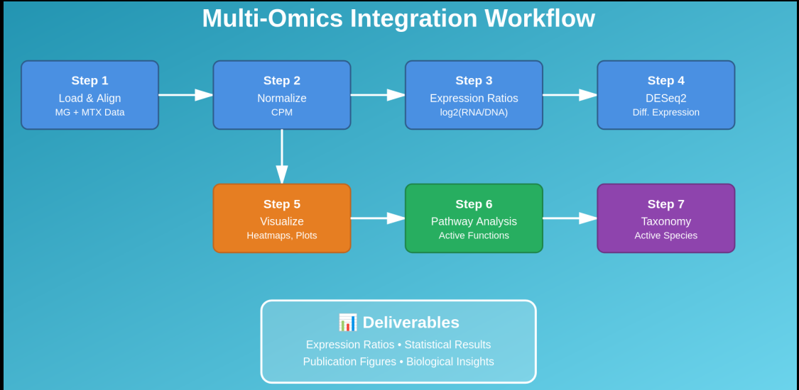
🧭 Workflow at a Glance (DNA + RNA Integration)
- MG (DNA) raw counts → CPM (for comparability)
- MTX (RNA) raw counts → DESeq2 (stats) + CPM (ratios/plots)
- Gene activity:
log2((RNA+1)/(DNA+1)) - Visual QC: histogram, MA plot, boxplot
- Higher-level integration: pathways + taxonomy → “active functions” & “active taxa”
🧬 Part 1: Introduction to Multi-Omics Integration
Why Integrate Metagenomics and Metatranscriptomics?
| Data Type | What It Tells Us | Limitation |
|---|---|---|
| Metagenomics (DNA) | Who’s present? What can they do? | Doesn’t show actual activity |
| Metatranscriptomics (RNA) | What are they actually doing? | Hard to assign to specific organisms |
| Integrated (DNA + RNA) | Active organisms + their functions | Complete functional picture! |
Key Questions Answered by Integration
- Which pathways are active beyond what genomic potential suggests?
- Which microbes are dormant vs actively functioning?
- How does community respond to environmental changes?
- What metabolic processes are upregulated or downregulated?
The Expression Ratio Concept
Expression Ratio = RNA abundance / DNA abundance

High ratio (>1): Gene is highly expressed relative to its abundance
Low ratio (<1): Gene is under-expressed despite being present
Ratio ≈ 1: Expression matches genomic potential
📊 Part 2: Data Preparation
Required Input Files
Before starting, we assume that we have the following data:
project/
├── metagenomics/
│   ├── gene_abundance_table.tsv      # Gene counts from MG
│   ├── pathway_abundance_table.tsv   # Pathway abundances from MG
│   └── taxonomy_abundance.tsv        # Taxonomic profiles from MG
├── metatranscriptomics/
│   ├── transcript_counts.tsv         # Transcript counts from MTX
│   ├── pathway_abundance_table.tsv   # Pathway abundances from MTX
│   └── taxonomy_abundance.tsv        # Taxonomic profiles from MTX
└── metadata.csv                      # Sample information
Setting Up Environment
# Create project structure
mkdir -p ~/multi_omics_integration/{data,scripts,results,figures}
cd ~/multi_omics_integration

# Install required R packages
R -e "install.packages(c('BiocManager', 'tidyverse', 'pheatmap', 'ggplot2', 'corrplot'))"
R -e "BiocManager::install(c('DESeq2', 'EnhancedVolcano', 'ComplexHeatmap'))"

# Install Python packages
pip install pandas numpy scipy matplotlib seaborn scikit-learn networkx --break-system-packages
Example Metadata File
Create metadata.csv:
SampleID,Condition,Timepoint,Replicate
Sample1_MG,Control,Day0,1
Sample2_MG,Control,Day0,2
Sample3_MG,Control,Day0,3
Sample4_MG,Treatment,Day7,1
Sample5_MG,Treatment,Day7,2
Sample6_MG,Treatment,Day7,3
Sample1_MTX,Control,Day0,1
Sample2_MTX,Control,Day0,2
Sample3_MTX,Control,Day0,3
Sample4_MTX,Treatment,Day7,1
Sample5_MTX,Treatment,Day7,2
Sample6_MTX,Treatment,Day7,3
🔗 Part 3: Gene-Level Integration
Python Scripts for Gene Expression Integration
Overview
Four standalone Python scripts that perform step-by-step integration of metagenomics (DNA) and metatranscriptomics (RNA) data to identify active genes and metabolic pathways. Please find all scripts in repo Day 10
Script 1: Load and Prepare Data
File: 01_load_and_prepare_data.py
What it does:
Loads raw count tables from metagenomics and metatranscriptomics experiments, identifies genes present in both datasets, and creates aligned matrices for fair comparison.
Key functions:
- Reads TSV/CSV count tables
- Finds overlapping genes between MG and MTX
- Filters datasets to common genes only
- Reports data quality metrics
Output:
- Aligned gene count matrices
- Summary statistics (genes, samples, overlap)
When to use:
First step of any multi-omics integration analysis
Script 2: Normalize Data
File: 02_normalize_data.py
What it does:
Converts raw counts to CPM (Counts Per Million) to account for differences in sequencing depth between samples. Essential for comparing samples with different library sizes.
Key functions:
- CPM normalization:
(count / total_reads) × 1,000,000 - Validates normalization (all samples = 1M)
- Reports sequencing depth statistics
Output:
- CPM-normalized gene abundance tables
- Sequencing depth summary
When to use:
After loading data, before calculating ratios
Why it matters:
Without normalization, a sample with 10M reads appears 2x more abundant than a sample with 5M reads, even if biological abundance is identical.
Script 3: Calculate Expression Ratios
File: 03_calculate_expression_ratios.py
What it does:
Calculates log2(RNA/DNA) ratios for each gene to identify which genes are more (or less) expressed than expected based on their genomic abundance.
Key functions:
- Computes
log2((RNA + 1) / (DNA + 1))for each gene - Identifies highly expressed genes (ratio > 2 = 4x more RNA)
- Identifies under-expressed genes (ratio < -2)
- Calculates mean and variability across samples
Output:
- Complete expression ratio matrix
- List of highly expressed genes
- List of under-expressed genes
- Summary statistics
When to use:
Core integration step after normalization
Interpretation:
- Ratio > 2: Active metabolism, stress response
- Ratio ≈ 0: Expression matches abundance
- Ratio < -2: Dormancy, energy conservation
Script 4: Visualize Expression Ratios
File: 04_visualize_expression_ratios.py
What it does:
Creates three publication-quality figures to visualize expression patterns across all genes and samples.
Figures generated:
- Histogram (
expression_ratio_histogram.png)- Shows distribution of expression ratios
- Identifies overall community activity
- Reference lines at key thresholds (0, 2)
- MA Plot (
ma_plot_expression.png)- X-axis: Gene abundance (DNA + RNA average)
- Y-axis: Expression ratio (RNA/DNA)
- Reveals if low/high abundance genes behave differently
- Detects technical biases
- Boxplot (
expression_ratio_boxplot.png)- Compares expression ratios across samples
- Shows sample-to-sample variability
- Identifies outlier samples
Output:
- Three high-resolution PNG figures (300 DPI)
- Ready for publication or presentations
When to use:
Final step for visual interpretation and quality control
Running the Scripts
Sequential execution:
python3 01_load_and_prepare_data.py
python3 02_normalize_data.py
python3 03_calculate_expression_ratios.py
python3 04_visualize_expression_ratios.py
Quick Reference Table
| Script | Input | Output | Purpose |
|---|---|---|---|
| 01 | Raw count tables | Aligned matrices | Prepare datasets |
| 02 | Aligned matrices | CPM-normalized data | Account for sequencing depth |
| 03 | Normalized data | Expression ratios | Identify active genes |
| 04 | Expression ratios | Figures (PNG) | Visualize patterns |
Expected Outputs Summary
After running all scripts, you’ll have:
Data files:
-
mg_genes_aligned.csv- Metagenomics aligned -
mtx_transcripts_aligned.csv- Metatranscriptomics aligned -
mg_genes_cpm.csv- MG normalized to CPM -
mtx_transcripts_cpm.csv- MTX normalized to CPM -
expression_ratios.csv- Complete ratio matrix -
highly_expressed_genes.csv- Top active genes -
under_expressed_genes.csv- Dormant genes
Figures:
expression_ratio_histogram.pngma_plot_expression.pngexpression_ratio_boxplot.png
Next Steps
After running these scripts:
- Review highly expressed genes for biological significance
- Perform functional enrichment analysis (KEGG, GO)
- Run DESeq2 for statistical differential expression
- Create pathway-level and taxonomic-level integrations
- Generate comprehensive multi-omics reports
These scripts lay the foundation for deeper multi-omics analysis!
📈 Part 4: Differential Expression Analysis with DESeq2
Why DESeq2 for Metatranscriptomics?
DESeq2 is designed for RNA-seq data and handles:
- Count data normalization
- Variance estimation across replicates
- Statistical testing for differential expression
- Multiple testing correction
Step 1: Prepare Count Matrix for DESeq2
import pandas as pd

# Load raw transcript counts (not normalized)
mtx_raw = pd.read_csv('data/transcript_counts.tsv', sep='\t', index_col=0)

# Filter low-abundance genes (at least 10 reads across all samples)
gene_sums = mtx_raw.sum(axis=1)
mtx_filtered = mtx_raw[gene_sums >= 10]

print(f"Genes before filtering: {mtx_raw.shape[0]}")
print(f"Genes after filtering: {mtx_filtered.shape[0]}")

# Save filtered count matrix
mtx_filtered.to_csv('results/mtx_counts_filtered.csv')

# Load and prepare metadata
metadata = pd.read_csv('metadata.csv', index_col=0)
metadata_mtx = metadata[metadata.index.str.contains('MTX')]

# Ensure sample order matches
mtx_filtered = mtx_filtered[metadata_mtx.index]

# Save metadata for R
metadata_mtx.to_csv('results/metadata_mtx.csv')

print("\nData prepared for DESeq2!")
Step 2: Run DESeq2 Analysis in R
Please see deseq2_analysis.R in Day 10**
Run the R script:
⚠️ Important: DESeq2 must use raw integer counts (not CPM/TPM/RPKM).
CPM is great for visualization and ratio-style summaries, but statistical DE testing should stay in DESeq2.
🔥 Part 5: Comparative Analysis- DNA vs RNA Abundance
🧰 Day 10 Scripts (Quick Index)
| Step | Script | Purpose | Outputs |
|---|---|---|---|
| 1 | 01_load_and_prepare_data.py | Align MG/MTX gene tables | aligned matrices |
| 2 | 02_normalize_data.py | CPM normalization | *_cpm.csv |
| 3 | 03_calculate_expression_ratios.py | log2(RNA/DNA) ratios | expression_ratios.csv |
| 4 | 04_visualize_expression_ratios.py | QC + overview plots | histogram, MA, boxplot |
| 5 | comparative_heatmaps.py | DNA vs RNA heatmaps | comparison PNG |
| 6 | ratio_heatmap.py | ratio heatmap of top genes | ratio heatmap PNG |
| 7 | pathway.py | pathway DNA vs RNA activity | pathway ratios + barplots |
| 8 | taxonomy_integration.py | taxa abundance vs activity | activity scores + plots |
Day 10 scripts comes with toy data for practicing Day 10
🎯 Part 8: Biological Interpretation Guide
Understanding Your Results
Expression Ratio Interpretation
| Log2(RNA/DNA) | Interpretation | Biological Meaning |
|---|---|---|
| > 3 | Very highly active | Stress response, active metabolism |
| 2 to 3 | Highly active | Active growth, core functions |
| 0 to 2 | Moderately active | Steady-state metabolism |
| -1 to 0 | Slightly under-expressed | Energy conservation |
| < -2 | Under-expressed | Dormancy, unfavorable conditions |
Common Biological Patterns
- High DNA + High RNA: Core metabolic genes, abundant active populations
- Low DNA + High RNA: Induced stress responses, specific adaptations
- High DNA + Low RNA: Dormant populations, genetic potential not utilized
- Low DNA + Low RNA: Rare inactive functions
Example Interpretation
Finding: Nitrogen fixation genes show high expression ratios (log2 = 3.5)
         but low genomic abundance (0.5% of community)

Interpretation: Although nitrogen-fixing bacteria are rare in the community,
                they are highly active, suggesting nitrogen limitation and
                an important ecological role for these minority members.
✅ Deliverables Checklist
- Expression ratios calculated for all genes
- DESeq2 differential expression analysis complete
- Comparative heatmaps (DNA vs RNA) generated
- Pathway activity analysis complete
- Taxonomic activity scores calculated
- All visualization figures saved
- Summary statistics report generated
- Biological interpretation written
🎉 Conclusion
Congratulations! You’ve now integrated metagenomics and metatranscriptomics data to:
- Identify which genes and pathways are actively expressed
- Discover which microbes are metabolically active
- Quantify differential expression between conditions
- Create publication-quality visualizations
Next Steps:
- Apply these methods to your own data
- Explore temporal multi-omics (time-series)
- Integrate with meta-metabolomics data
- Investigate strain-level activity patterns
Remember: Integration reveals the complete functional story - who’s there (DNA), what they’re doing (RNA), and how they respond to their environment!
Repo for today’s code and other details
🔗 Day 10
Last updated: February 2026