Day 1: Quality Control, Contamination Removal, and Read-Based Taxonomic Analysis
Day 1: Quality Control, Contamination Removal, and Read-Based Taxonomic Analysis
Table of Contents
- Introduction
- Prerequisites
- Workflow Overview
- Quality Control with FastQC
- Aggregating QC Reports with MultiQC
- Adapter Trimming and Quality Filtering
- Host and Contaminant Removal
- PhiX Removal
- Read-Based Taxonomic Profiling
- Comparing Results
- Best Practices and Tips
- Troubleshooting
- Next Steps
Introduction
Welcome to Day 1 of our comprehensive metagenome analysis series! Before we can assemble genomes or identify microbial functions, we need to ensure our raw sequencing data is of high quality and free from contamination.
In shotgun metagenomic sequencing, we sequence all the DNA present in an environmental sample. This approach gives us access to:
- Complete genomes of microorganisms (not just marker genes like 16S rRNA)
- All genes including those involved in metabolism, antibiotic resistance, virulence
- Functional potential of the microbial community
However, raw sequencing data often contains:
- Low-quality bases
- Adapter sequences from library preparation
- Host DNA (human, mouse, plant, etc.)
- PhiX control sequences (Illumina sequencing spike-in)
- Environmental contaminants
Today’s tutorial will guide you through cleaning and profiling your metagenomic data before assembly.
Prerequisites
Required Software
# Quality Control
- FastQC (v0.11.9 or higher)
- MultiQC (v1.12 or higher)

# Read Processing
- Trimmomatic (v0.39 or higher)
- BBTools (BBDuk) (v38.90 or higher)
- KneadData (v0.12.0 or higher)

# Taxonomic Profiling
- Kaiju (v1.9.0 or higher)
- Kraken2 (v2.1.2 or higher)
- Bracken (v2.7 or higher)
- mOTUs (v3.0.3 or higher)
- MetaPhlAn (v4.0 or higher)
Computational Resources
- Minimum: 16 GB RAM, 8 cores
- Recommended: 64 GB RAM, 32 cores
- Storage: 100 GB for databases + 50 GB per sample
Database Preparation
You’ll need to download reference databases for taxonomic profiling. This can take several hours.
Running on Different Platforms
Note: This tutorial is primarily designed for HPC (High-Performance Computing) environments where you have access to significant computational resources. However, you can absolutely learn and practice metagenome analysis on your personal desktop! Below are platform-specific guidelines.
🖥️ For Personal Desktop Users
If you’re learning metagenomics on your personal computer, here are some considerations and modifications:
Hardware Requirements by Platform
Minimum for Learning (Small datasets):
- RAM: 8 GB (can process subsampled data)
- CPU: 4 cores
- Storage: 50 GB free space
- Dataset size: Subsample to 1-5 million read pairs
Recommended for Real Analysis:
- RAM: 32 GB
- CPU: 8+ cores
- Storage: 500 GB+ SSD
- Dataset size: Full metagenomes
🐧 Linux Desktop Installation
Linux is the most straightforward platform for bioinformatics. Most tools have native Linux support.
Option 1: Using Conda (Recommended)
# Install Miniconda (if not already installed)
wget https://repo.anaconda.com/miniconda/Miniconda3-latest-Linux-x86_64.sh
bash Miniconda3-latest-Linux-x86_64.sh

# Create environment for Day 1 tools
conda create -n metagenomics_day1 python=3.9
conda activate metagenomics_day1

# Install all tools at once
conda install -c bioconda -c conda-forge \
    fastqc \
    multiqc \
    trimmomatic \
    bbmap \
    kneaddata \
    kaiju \
    kraken2 \
    bracken \
    motus \
    metaphlan

# Verify installations
fastqc --version
kraken2 --version
Option 2: Manual Installation
# FastQC
sudo apt-get update
sudo apt-get install fastqc

# Trimmomatic
wget http://www.usadellab.org/cms/uploads/supplementary/Trimmomatic/Trimmomatic-0.39.zip
unzip Trimmomatic-0.39.zip
echo 'alias trimmomatic="java -jar /path/to/Trimmomatic-0.39/trimmomatic-0.39.jar"' >> ~/.bashrc

# BBTools
wget https://sourceforge.net/projects/bbmap/files/latest/download -O BBMap.tar.gz
tar -xzf BBMap.tar.gz
echo 'export PATH=$PATH:/path/to/bbmap' >> ~/.bashrc
source ~/.bashrc
Desktop-Specific Tips for Linux
# Adjust thread count for desktop (use n-1 cores)
THREADS=$(nproc --all)
THREADS=$((THREADS - 1))

# Subsample large files for testing
seqtk sample -s100 large_file_R1.fastq.gz 1000000 | gzip > small_R1.fastq.gz
seqtk sample -s100 large_file_R2.fastq.gz 1000000 | gzip > small_R2.fastq.gz

# Monitor resources
htop  # Install with: sudo apt-get install htop
🍎 macOS Installation
macOS is Unix-based, so most Linux tools work with minor adjustments.
Using Conda (Recommended)
# Install Homebrew (if not already installed)
/bin/bash -c "$(curl -fsSL https://raw.githubusercontent.com/Homebrew/install/HEAD/install.sh)"

# Install Miniconda via Homebrew
brew install --cask miniconda

# Initialize conda
conda init zsh  # or 'bash' if using bash

# Create environment (same as Linux)
conda create -n metagenomics_day1 python=3.9
conda activate metagenomics_day1

# Install tools
conda install -c bioconda -c conda-forge \
    fastqc multiqc trimmomatic bbmap \
    kaiju kraken2 bracken motus metaphlan
macOS-Specific Considerations
# Java for Trimmomatic (if needed)
brew install openjdk@11
echo 'export PATH="/usr/local/opt/openjdk@11/bin:$PATH"' >> ~/.zshrc

# Use all cores except 2 (leave some for system)
THREADS=$(sysctl -n hw.ncpu)
THREADS=$((THREADS - 2))

# Check memory before running
vm_stat | head -n 10
Known macOS Issues and Solutions
# If you encounter "command not found" after conda install
conda activate metagenomics_day1
which fastqc  # Should show conda path

# If Java version conflicts (for Trimmomatic)
export JAVA_HOME=$(/usr/libexec/java_home -v 11)

# M1/M2 Mac users: Some tools need Rosetta 2
softwareupdate --install-rosetta
🪟 Windows Installation (WSL2 Recommended)
Running bioinformatics tools natively on Windows is challenging. Windows Subsystem for Linux 2 (WSL2) is the best solution.
Step 1: Install WSL2
# Open PowerShell as Administrator and run:
wsl --install -d Ubuntu-22.04

# Restart your computer

# After restart, set up Ubuntu username and password
Step 2: Set Up Ubuntu in WSL2
# Update Ubuntu
sudo apt update && sudo apt upgrade -y

# Install essential build tools
sudo apt install -y build-essential curl wget git

# Install Miniconda
wget https://repo.anaconda.com/miniconda/Miniconda3-latest-Linux-x86_64.sh
bash Miniconda3-latest-Linux-x86_64.sh
source ~/.bashrc

# Install tools (same as Linux)
conda create -n metagenomics_day1 python=3.9
conda activate metagenomics_day1
conda install -c bioconda -c conda-forge \
    fastqc multiqc trimmomatic bbmap \
    kaiju kraken2 bracken motus metaphlan
Step 3: Access Windows Files from WSL2
# Your Windows C: drive is at /mnt/c/
cd /mnt/c/Users/YourUsername/Documents/metagenomics

# Or create a working directory in WSL2
mkdir -p ~/metagenomics_project
cd ~/metagenomics_project
Windows-Specific Tips
# Find optimal thread count (in WSL2)
THREADS=$(nproc --all)
THREADS=$((THREADS / 2))  # WSL2 typically gets half of Windows cores

# Set memory limit for WSL2
# Create file: C:\Users\YourUsername\.wslconfig
# Add these lines:
[wsl2]
memory=16GB
processors=8
swap=8GB

# Restart WSL2
wsl --shutdown
Alternative: Docker Desktop on Windows
# After installing Docker Desktop with WSL2 backend

# Pull a bioinformatics image
docker pull quay.io/biocontainers/fastqc:0.11.9--0

# Run FastQC
docker run -v ${PWD}:/data quay.io/biocontainers/fastqc:0.11.9--0 \
    fastqc /data/*.fastq.gz -o /data/qc_results
💾 Working with Limited Resources
If you have a personal desktop with limited RAM/CPU, here are strategies:
1. Subsample Your Data
# Install seqtk
conda install -c bioconda seqtk

# Subsample to 1 million read pairs (for learning)
seqtk sample -s100 original_R1.fastq.gz 1000000 > subset_R1.fastq
seqtk sample -s100 original_R2.fastq.gz 1000000 > subset_R2.fastq
gzip subset_R*.fastq

# This gives you ~300 MB files instead of 10+ GB
2. Use Lighter-Weight Tools
# Instead of Kraken2 Standard (50GB database):
# Use Kraken2 MiniKraken (8GB database)
wget https://genome-idx.s3.amazonaws.com/kraken/minikraken2_v2_8GB_201904.tgz
tar -xzf minikraken2_v2_8GB_201904.tgz

# Instead of Kaiju nr (70GB):
# Use Kaiju RefSeq (30GB) or PROGENOMES (15GB)
kaiju-makedb -s refseq
3. Process Samples Sequentially
# Instead of parallel processing:
for sample in sample1 sample2 sample3; do
    echo "Processing ${sample}..."
    # Run your analysis here
    # One sample at a time
done
4. Use Cloud-Free Alternatives for Large Steps
# Skip host removal if working with environmental samples
# (less critical than for human gut/skin samples)

# Use read-based taxonomy only (skip assembly until Day 2)
# This is sufficient for community profiling
📚 Recommended Learning Workflow for Desktop Users
Week 1: Start Small
# Use tutorial datasets (small, ~100MB)
wget http://example.com/tutorial_dataset.tar.gz

# Practice all QC steps
# Get familiar with FastQC reports
# Understand trimming parameters
Week 2: Scale Up
# Subsample real data to 5M reads
# Run full QC pipeline
# Try different taxonomic profilers
Week 3: Full Dataset
# Process complete dataset (if resources allow)
# Or move to HPC/cloud for this step
🌐 Cloud Alternatives
If your desktop is insufficient, consider:
- Google Colab (Free, 12GB RAM)
- Upload small datasets
- Run FastQC, Trimmomatic
- Good for learning
- AWS Free Tier
- 750 hours/month of t2.micro
- Scale up when needed
- Galaxy Public Servers (Covered in Day 8)
- No installation needed
- Web-based interface
- Free for academic use
🔧 Platform Comparison Summary
| Feature | HPC | Linux Desktop | macOS | Windows (WSL2) |
|---|---|---|---|---|
| Ease of Setup | ⭐⭐⭐⭐ | ⭐⭐⭐⭐⭐ | ⭐⭐⭐⭐ | ⭐⭐⭐ |
| Performance | ⭐⭐⭐⭐⭐ | ⭐⭐⭐ | ⭐⭐⭐ | ⭐⭐ |
| Tool Compatibility | ⭐⭐⭐⭐⭐ | ⭐⭐⭐⭐⭐ | ⭐⭐⭐⭐ | ⭐⭐⭐⭐ |
| Learning Friendly | ⭐⭐⭐ | ⭐⭐⭐⭐⭐ | ⭐⭐⭐⭐ | ⭐⭐⭐⭐ |
| Cost | Varies | Free | Free | Free |
Recommendation:
- Learning: Linux desktop or WSL2
- Production: HPC or Cloud
- Mac users: Great for learning, may need cloud for large datasets
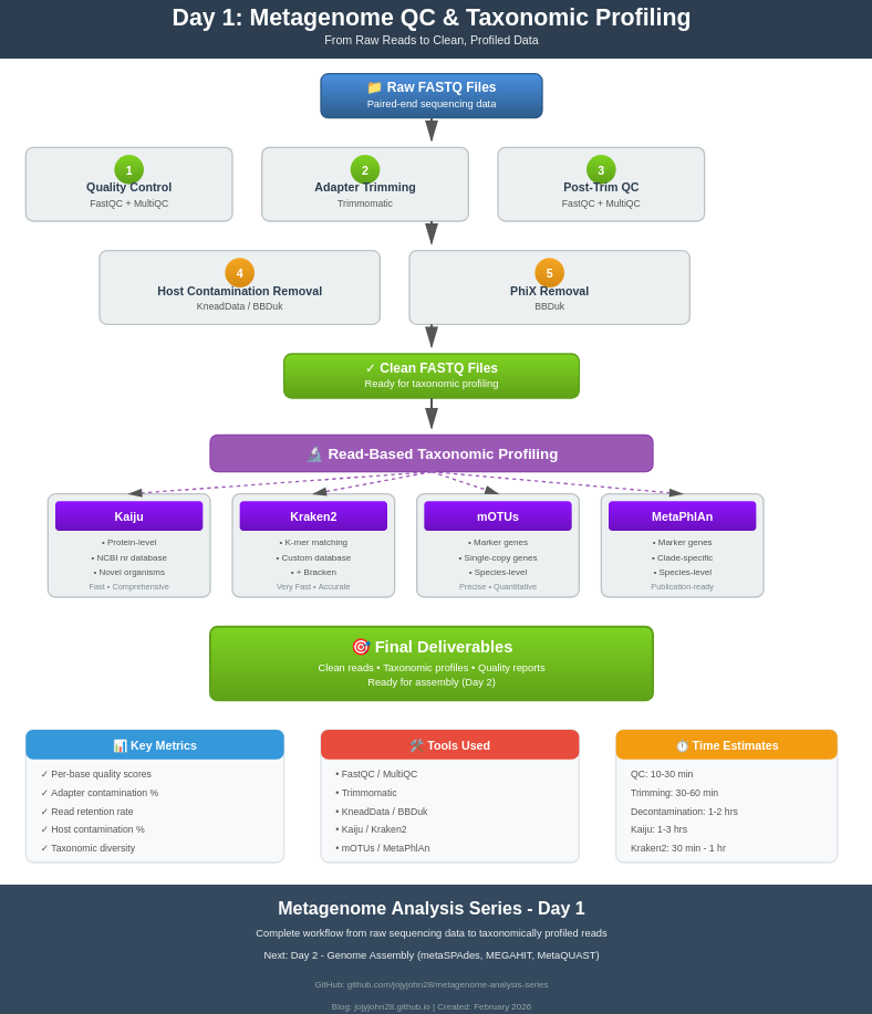
Workflow Overview
Raw FASTQ files
    ↓
1. FastQC (initial quality check)
    ↓
2. MultiQC (aggregate reports)
    ↓
3. Trimmomatic (adapter removal, quality trimming)
    ↓
4. FastQC (post-trimming QC)
    ↓
5. KneadData/BBDuk (host and PhiX removal)
    ↓
6. FastQC (final QC check)
    ↓
7. Read-based taxonomic profiling
   - Kaiju (protein-level)
   - Kraken2 + Bracken (k-mer based)
   - mOTUs (marker gene)
   - MetaPhlAn (marker gene)
    ↓
Clean, profiled reads ready for assembly
Quality Control with FastQC
FastQC provides a quick overview of your sequencing data quality. It generates reports with various quality metrics.
Running FastQC
# Navigate to your working directory
cd /path/to/your/project
mkdir -p qc/fastqc_raw

# Load FastQC (if using a module system like on HPC)
module load fastqc/0.11.9

# Run FastQC on all raw FASTQ files
fastqc -o qc/fastqc_raw \
       -t 8 \
       -f fastq \
       raw_data/*.fastq.gz

# Options explained:
# -o : Output directory
# -t : Number of threads (parallel processing)
# -f : Input file format
Understanding FastQC Reports
Open the HTML files in qc/fastqc_raw/ to view the reports. Key sections to check:
1. Per Base Sequence Quality
- Good: Phred scores >28 (green zone) across all bases
- Warning: Scores between 20-28 (orange zone)
- Fail: Scores <20 (red zone)
- What to look for: Quality typically drops at the 3’ end of reads
2. Per Sequence Quality Scores
- Most reads should have mean quality >30
- Low-quality reads (mean <20) indicate sequencing issues
3. Per Base Sequence Content
- In random libraries, A/T/G/C should be roughly equal (~25% each)
- First 10-15 bases may show bias (library prep artifacts)
- For metagenomes: Some variation is normal due to diverse organisms
4. Sequence Duplication Levels
- High duplication may indicate PCR artifacts or low complexity samples
- For metagenomes: Some duplication is expected (high-abundance organisms)
5. Adapter Content
- Should be minimal (<5%)
- If present, needs trimming
6. Overrepresented Sequences
- May indicate contaminants, adapters, or highly abundant organisms
Running FastQC on Multiple Samples
For batch processing multiple samples, see the shell script: 01_fastqc_batch.sh
Aggregating QC Reports with MultiQC
MultiQC combines reports from multiple samples and tools into a single interactive HTML report.
Installation
# Using pip
pip install multiqc

# Using conda
conda install -c bioconda multiqc
Running MultiQC
# Aggregate all FastQC reports
multiqc qc/fastqc_raw \
        -o qc/multiqc_raw \
        -n raw_reads_report

# Options:
# -o : Output directory
# -n : Report name
Interpreting MultiQC Reports
The MultiQC report provides:
- General Statistics: Read counts, %GC, %duplicates across all samples
- Sequence Quality Histograms: Compare quality across samples
- Adapter Content: Identify samples needing aggressive trimming
- Sample Clustering: Detect outlier samples
Red flags to watch for:
- Samples with <1 million reads (may have low coverage)
- Mean quality <25 (poor sequencing run)
-
20% adapter content (need trimming)
- Extreme %GC deviation (contamination or extraction issues)
Adapter Trimming and Quality Filtering
After initial QC, we remove adapter sequences and low-quality bases using Trimmomatic.
Trimmomatic Overview
Trimmomatic performs several operations in a specific order:
- Remove Illumina adapters (ILLUMINACLIP)
- Remove leading low-quality bases (LEADING)
- Remove trailing low-quality bases (TRAILING)
- Scan with sliding window (SLIDINGWINDOW)
- Drop reads below minimum length (MINLEN)
Basic Trimmomatic Command
# Single sample, paired-end
java -jar /path/to/trimmomatic-0.39.jar PE \
     -threads 8 \
     -phred33 \
     raw_data/sample1_R1.fastq.gz \
     raw_data/sample1_R2.fastq.gz \
     trimmed/sample1_R1_paired.fastq.gz \
     trimmed/sample1_R1_unpaired.fastq.gz \
     trimmed/sample1_R2_paired.fastq.gz \
     trimmed/sample1_R2_unpaired.fastq.gz \
     ILLUMINACLIP:adapters/TruSeq3-PE.fa:2:30:10:2:True \
     LEADING:3 \
     TRAILING:3 \
     SLIDINGWINDOW:4:15 \
     MINLEN:36

# PE: Paired-end mode
# -threads: Number of CPU threads
# -phred33: Quality score encoding (standard for Illumina 1.8+)
Understanding Trimmomatic Parameters
ILLUMINACLIP Parameters
ILLUMINACLIP:TruSeq3-PE.fa:2:30:10:2:True
                         │  │  │  │ └─ keepBothReads
                         │  │  │  └─── minAdapterLength
                         │  │  └────── simpleClipThreshold
                         │  └───────── palindromeClipThreshold
                         └──────────── seedMismatches
- seedMismatches (2): Maximum mismatches in seed alignment
- palindromeClipThreshold (30): Threshold for palindrome alignment (paired reads)
- simpleClipThreshold (10): Threshold for simple alignment (single read)
- minAdapterLength (2): Minimum adapter length to detect
- keepBothReads (True): Keep both reads even if adapter in only one
Quality Trimming Parameters
LEADING:3      # Remove leading bases with quality < 3
TRAILING:3     # Remove trailing bases with quality < 3
SLIDINGWINDOW:4:15  # Window size:quality threshold
MINLEN:36      # Minimum read length after trimming
Recommended settings for metagenomics:
- Conservative (high quality): SLIDINGWINDOW:4:20, MINLEN:50
- Standard: SLIDINGWINDOW:4:15, MINLEN:36
- Aggressive (maximize retention): SLIDINGWINDOW:4:10, MINLEN:30
Batch Processing with Trimmomatic
For processing multiple samples, see: 02_trimmomatic_batch.sh
The script also generates a summary CSV file with trimming statistics.
Post-Trimming QC
# Run FastQC on trimmed reads
mkdir -p qc/fastqc_trimmed

fastqc -o qc/fastqc_trimmed \
       -t 8 \
       trimmed/*_paired.fastq.gz

# Generate MultiQC report
multiqc qc/fastqc_trimmed \
        -o qc/multiqc_trimmed \
        -n trimmed_reads_report
Host and Contaminant Removal
Metagenomic samples often contain host DNA (human, mouse, plant, etc.) that needs to be removed before analysis. We’ll use KneadData or BBDuk for this step.
Option 1: KneadData (Recommended)
KneadData is specifically designed for metagenomic data and integrates multiple tools.
Installation
# Using conda (recommended)
conda create -n kneaddata -c bioconda kneaddata
conda activate kneaddata

# Download human reference database (GRCh38)
kneaddata_database --download human_genome bowtie2 /path/to/databases/kneaddata_db
Running KneadData
mkdir -p decontaminated
mkdir -p logs/kneaddata

# Single sample
kneaddata \
    --input trimmed/sample1_R1_paired.fastq.gz \
    --input trimmed/sample1_R2_paired.fastq.gz \
    --output decontaminated/sample1 \
    --reference-db /path/to/databases/kneaddata_db/human_genome \
    --threads 16 \
    --trimmomatic /path/to/trimmomatic \
    --bypass-trim \
    --log logs/kneaddata/sample1.log

# Options:
# --bypass-trim : Skip trimming (already done with Trimmomatic)
# --reference-db : Path to host genome database
# --threads : Number of threads
Batch Processing with KneadData
For batch processing, see: 03_kneaddata_batch.sh
Option 2: BBDuk (Fast alternative)
BBDuk from BBTools is faster and uses less memory than KneadData.
Installation
# Download BBTools
wget https://sourceforge.net/projects/bbmap/files/latest/download -O BBMap.tar.gz
tar -xzf BBMap.tar.gz
export PATH=$PATH:/path/to/bbmap
Download Host Reference
# Download human genome
wget https://ftp.ncbi.nlm.nih.gov/genomes/all/GCA/000/001/405/GCA_000001405.15_GRCh38/GCA_000001405.15_GRCh38_genomic.fna.gz
gunzip GCA_000001405.15_GRCh38_genomic.fna.gz
mv GCA_000001405.15_GRCh38_genomic.fna human_ref.fna
Running BBDuk for Host Removal
For batch processing, see: 04_bbduk_host_removal.sh
PhiX Removal
PhiX is a control DNA added by Illumina during sequencing. It must be removed before analysis.
Using BBDuk for PhiX Removal
For batch processing, see: 05_phix_removal.sh
Combined Host and PhiX Removal
You can remove both host and PhiX in a single step:
# Concatenate references
cat databases/human_ref.fna bbmap/resources/phix174_ill.ref.fa.gz > databases/contaminants.fna

# Run BBDuk once
bbduk.sh \
    in1=trimmed/sample1_R1_paired.fastq.gz \
    in2=trimmed/sample1_R2_paired.fastq.gz \
    out1=clean/sample1_R1_clean.fastq.gz \
    out2=clean/sample1_R2_clean.fastq.gz \
    ref=databases/contaminants.fna \
    k=31 \
    hdist=1 \
    threads=16
Final QC Check
Run FastQC and MultiQC on final cleaned reads, then generate a read count summary. See: 06_final_qc_summary.sh
Read-Based Taxonomic Profiling
Now that we have clean reads, we can identify the organisms present in our samples. We’ll use multiple tools to get a comprehensive view.
Tool Comparison
| Tool | Database | Approach | Speed | Memory | Best For |
|---|---|---|---|---|---|
| Kaiju | NCBI nr (proteins) | Protein alignment | Fast | Medium | Comprehensive, novel organisms |
| Kraken2 | Custom (DNA) | K-mer matching | Very Fast | High | Speed, abundance estimation |
| Bracken | Uses Kraken2 | Statistical | Fast | Low | Abundance refinement |
| mOTUs | Marker genes | Gene alignment | Medium | Low | Species-level precision |
| MetaPhlAn | Marker genes | Marker alignment | Medium | Low | Species-level, publication-ready |
1. Kaiju (Protein-based classification)
Kaiju uses protein-level alignment against NCBI’s nr database, making it sensitive to novel or divergent organisms.
Database Setup
# Create database directory
mkdir -p databases/kaiju
cd databases/kaiju

# Download and build database (choose one)
# Option 1: nr database (comprehensive, ~70GB, takes hours)
kaiju-makedb -s nr

# Option 2: RefSeq (smaller, faster, ~30GB)
kaiju-makedb -s refseq

# Option 3: PROGENOMES (small, for bacteria/archaea only, ~15GB)
kaiju-makedb -s progenomes

# This creates:
# - kaiju_db_*.fmi (index file)
# - nodes.dmp (taxonomy)
# - names.dmp (taxonomy names)
Running Kaiju
For batch processing with summary generation, see: 07_kaiju_profiling.sh
Understanding Kaiju Output
The .out file has columns:
- C/U - Classified (C) or Unclassified (U)
- Read ID
- NCBI TaxID - Taxonomic identifier
- Score - Match quality
- TaxIDs - Comma-separated list of matching taxa
- Accessions - Database accessions
- Fragment - Matching sequence
2. Kraken2 + Bracken (K-mer based classification)
Kraken2 is extremely fast and uses k-mer matching. Bracken refines abundance estimates to species level.
Database Setup
# Create database directory
mkdir -p databases/kraken2
cd databases/kraken2

# Option 1: Standard database (bacteria, archaea, viral, human, ~50GB)
kraken2-build --standard --threads 32 --db kraken2_standard

# Option 2: Custom database (recommended for metagenomics)
# Download NCBI taxonomy
kraken2-build --download-taxonomy --db kraken2_custom

# Download libraries (choose what you need)
kraken2-build --download-library bacteria --db kraken2_custom
kraken2-build --download-library archaea --db kraken2_custom
kraken2-build --download-library viral --db kraken2_custom
kraken2-build --download-library fungi --db kraken2_custom
kraken2-build --download-library protozoa --db kraken2_custom

# Build database
kraken2-build --build --threads 32 --db kraken2_custom

# Build Bracken database (for abundance estimation)
bracken-build -d databases/kraken2/kraken2_custom -t 32 -k 35 -l 150
Running Kraken2
For batch processing with Bracken abundance estimation, see: 08_kraken2_bracken.sh
Understanding Kraken2 Output
Kraken output (.kraken):
- Column 1: C/U (Classified/Unclassified)
- Column 2: Read ID
- Column 3: Taxonomy ID
- Column 4: Read length
- Column 5: LCA mapping
Kraken report (.report):
- Column 1: Percentage of reads
- Column 2: Number of reads (cumulative)
- Column 3: Number of reads (specific)
- Column 4: Taxonomic rank (U, D, K, P, C, O, F, G, S)
- Column 5: NCBI TaxID
- Column 6: Scientific name
3. mOTUs (Marker gene profiling)
mOTUs uses single-copy marker genes for species-level profiling with high precision.
Database Setup
# Install mOTUs
conda install -c bioconda motus

# Download database
motus downloadDB
Running mOTUs
For batch processing and merging profiles, see: 09_motus_profiling.sh
4. MetaPhlAn (Publication-ready marker gene profiling)
MetaPhlAn is widely used and produces publication-ready taxonomic profiles.
Database Setup
# Install MetaPhlAn
conda install -c bioconda metaphlan

# Database is automatically downloaded on first run
# Or manually download:
metaphlan --install --bowtie2db databases/metaphlan
Running MetaPhlAn
For batch processing and merging abundance tables, see: 10_metaphlan_profiling.sh
Comparing Results
Different tools may give different results. Here’s how to compare them:
Visualization with R
For comprehensive visualization including heatmaps, barplots, and comparisons across tools, see: compare_taxonomy.R
Venn Diagram of Detected Taxa
For comparing detected taxa across tools, see: 11_venn_diagram_taxa.sh
Best Practices and Tips
1. Quality Control
- Always check FastQC reports before and after each processing step
- Remove samples with <1M reads or mean quality <25
- Keep unpaired reads from Trimmomatic - they can still be useful
2. Contamination Removal
- Use the most specific host genome available (e.g., mouse strain if known)
- Check PhiX levels - high PhiX (>5%) indicates sequencing QC issues
- Keep removed reads for debugging (outm files)
3. Taxonomic Profiling
- Use multiple tools for validation
- Kaiju is best for novel/divergent organisms
- Kraken2 is fastest for routine analysis
- MetaPhlAn is best for publication
- Always check unclassified read percentages
4. Resource Management
- Use
screenortmuxfor long-running jobs - Compress intermediate files to save space
- Delete temporary files after verification
5. Documentation
- Keep a log of all commands
- Record software versions
- Save database versions and dates
Troubleshooting
Problem: Low read quality after trimming
Solution: Adjust SLIDINGWINDOW parameter or increase MINLEN
Problem: High percentage of host reads
Solution:
- Check extraction protocol
- Ensure correct host genome is used
- Consider enrichment strategies for low-biomass samples
Problem: High unclassified reads (>50%)
Possible causes:
- Novel organisms not in database
- Poor sequencing quality
- Contamination with non-biological sequences
- Wrong database (e.g., bacterial database for fungal sample)
Solutions:
- Use Kaiju with nr database (most comprehensive)
- Check FastQC for adapter/quality issues
- Update databases to latest versions
Problem: Inconsistent results between tools
This is normal! Different tools use different approaches:
- Focus on high-abundance taxa (>1%)
- Taxa detected by multiple tools are most reliable
- Use tool-specific strengths (Kaiju for discovery, MetaPhlAn for quantification)
Problem: Out of memory errors
Solutions:
- Reduce Kraken2 database size
- Use –memory-mapping flag with Kraken2
- Process samples sequentially instead of parallel
- Downsample reads for testing
Next Steps
Congratulations! You now have: ✅ High-quality, clean sequencing reads ✅ Host and contaminant-free data ✅ Taxonomic profiles of your samples
Tomorrow (Day 2), we’ll use these clean reads for:
- De novo assembly with metaSPAdes and MEGAHIT
- Assembly quality assessment with MetaQUAST
- Comparing assembly strategies
Prepare for Day 2:
- Review your taxonomic results
- Calculate total clean reads per sample
- Ensure you have sufficient storage (assemblies can be large!)
- Install assemblers:
conda install -c bioconda spades megahit quast
Summary
In this tutorial, we covered:
- ✅ Quality assessment with FastQC and MultiQC
- ✅ Adapter trimming and quality filtering with Trimmomatic
- ✅ Host genome removal with KneadData/BBDuk
- ✅ PhiX contamination removal
- ✅ Read-based taxonomic profiling with Kaiju, Kraken2, mOTUs, and MetaPhlAn
- ✅ Comparing and visualizing results
These cleaned reads are now ready for assembly and downstream analysis!
Additional Resources
Documentation
- FastQC Manual
- Trimmomatic Documentation
- KneadData Tutorial
- Kaiju GitHub
- Kraken2 Manual
- For more details , scripts and data visit: https://github.com/jojyjohn28/metagenome-analysis-series/tree/main/day1/
- Follow the blog for Day 2!
Happy metagenomic analyzing! 🧬