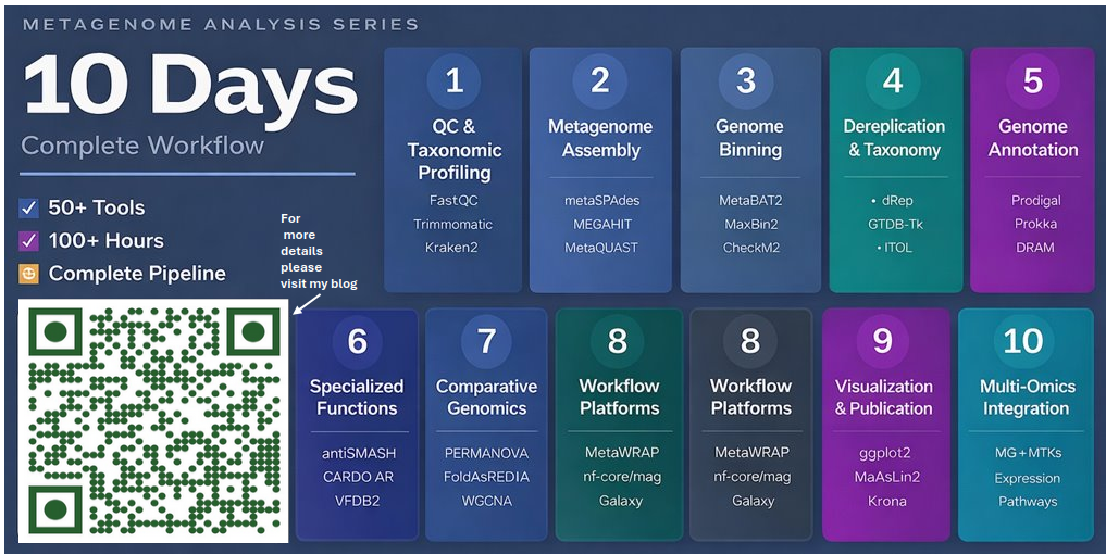
10-Day Metagenome Analysis Series - Complete Summary
Complete workflow from raw sequencing data to publication-ready insights
📊 Overview
Day 1: Metagenome QC & Taxonomic Profiling
From Raw Reads to Clean, Profiled Data
What You’ll Do:
- Quality control of raw sequencing reads
- Adapter trimming and host contamination removal
- Read-based taxonomic profiling
- PhiX removal
Key Tools:
- FastQC / MultiQC - Quality assessment
- Trimmomatic - Adapter trimming
- Kraken2 - K-mer matching taxonomy
- Kaiju - Protein-level classification
- MetaPhlAn - Marker gene profiling
- mOTUs - Universal marker genes
Time Estimate: 10-20 minutes (QC) + 30 min-1 hr (Taxonomy)
Deliverables:
- Clean FASTQ files
- Taxonomic profiles
- Quality reports
- Ready for assembly
📝 Day 1
📂 Metagenome Analysis Series Repo
Day 2: Metagenome Assembly
Reconstructing Genomes from Short Reads
What You’ll Do:
- Assemble clean reads into contigs
- Quality assessment of assemblies
- Calculate coverage
- Choose best assembler
Key Tools:
- metaSPAdes - Multi-k-mer assembly (high quality)
- MEGAHIT - Memory-efficient (fast)
- Flye - Long-read assembly
- MetaQUAST - Assembly quality assessment
- Bowtie2 - Read mapping
- SAMtools - Coverage calculation
Time Estimate: 6-12 hours (MEGAHIT: 2-8 hrs)
Deliverables:
- Assembled contigs (contigs.fasta)
- Quality reports (N50, L50, total length)
- Coverage files
- Ready for binning
📝 Day 2
📂 Metagenome Analysis Series Repo
Day 3: Genome Binning
Recovering Individual Genomes (MAGs) from Metagenomes
What You’ll Do:
- Bin contigs into individual genomes
- Refine bins using multiple binners
- Assess bin quality
- Profile abundance across samples
Key Tools:
- MetaBAT2 - Coverage-based binning
- MaxBin2 - Marker gene binning
- CONCOCT - Composition-based binning
- MetaWRAP - Bin refinement (combines all 3)
- CheckM2 - Quality assessment
- CoverM - Abundance profiling
- SingleM - Validation
Time Estimate: 12-24 hours total
- Initial binning: 4-8 hrs
- Refinement: 2-6 hrs
- Quality check: 1-2 hrs
- Abundance: 2-4 hrs
Quality Metrics:
- Completeness (target >50%, ideally >90%)
- Contamination (target <10%, ideally <5%)
- N50 (contig length)
Deliverables:
- High-quality MAGs (>50% complete, <10% contamination)
- Abundance tables
- Coverage metrics
- Ready for annotation
📝 Day 3
📂 Metagenome Analysis Series Repo
Day 4: Dereplication & Taxonomy
Identifying Unique Species and Classifying Genomes
What You’ll Do:
- Remove redundant/duplicate genomes
- Classify MAGs taxonomically
- Build phylogenetic trees
- Identify novel species
Key Tools:
- dRep - Dereplication (primary, 95% ANI for species)
- GTDB-Tk - GTDB taxonomy classification
- pyani - Average Nucleotide Identity
- iTOL - Interactive phylogenetic tree visualization
Time Estimate: 6-17 hours
- dRep (MASH + ANI): 1-4 hrs
- GTDB-Tk: 4-12 hrs (identify + classify)
- Visualization: 1 hr
Outputs:
- Species representatives (40-70% fewer genomes)
- Full GTDB taxonomy
- ANI matrices
- Phylogenetic trees
- Novel species identified (ANI <95%)
Success Rates:
- Classification: 95-99% success
- Novel species: 10-30% (ANI <95%)
- Novel genera: 1-5% (ANI <85%)
Deliverables:
- Dereplicated MAG set
- Complete taxonomy assignments
- Species catalog
- Phylogenetic trees
📝 Day 4
Day 5: Genome Annotation
Understanding Metabolic Potential
What You’ll Do:
- Predict genes in MAGs
- Annotate gene functions
- Map to metabolic pathways
- Identify biosynthetic potential
Key Tools:
- Prodigal - Gene prediction (100% genes)
- Prokka - Rapid annotation (60-80%)
- eggNOG-mapper - Functional annotation (70-90%)
- DRAM - Metabolic distillation (40-60% pathways)
- METABOLIC - Comprehensive pathways (40+ pathways)
Time Estimate: 3-4 hours (10 genomes)
- Prodigal: 5 min
- Prokka: 50 min
- eggNOG: 5 hrs
- DRAM: 3-4 hrs
Annotation Coverage:
- Genes predicted: 100% (Prodigal)
- Functions assigned: 60-80% (Prokka), 70-90% (eggNOG)
- Pathways identified: 40+ (METABOLIC)
Deliverables:
- Annotated gene files (.gbk, .gff, .faa)
- Functional summaries (KEGG, COG, GO, EC)
- Metabolic pathway maps
- Interactive diagrams
- Ready for comparative genomics
📝 Day 5
Day 6: Specialized Genomic Functions
Discovering Hidden Capabilities
What You’ll Do:
- Identify biosynthetic gene clusters (BGCs)
- Find antimicrobial resistance genes
- Detect CRISPR-Cas systems
- Identify prophages
- Discover mobile genetic elements
- Find protein domains
Key Tools:
- antiSMASH - Secondary metabolites (BGCs: 5-30 per genome)
- CARD-RGI - Antimicrobial resistance (AMR genes)
- ABRicate - Resistance gene screening
- dbCAN2 - Carbohydrate-active enzymes (CAZymes: 50-500)
- VirSorter2 - Prophage detection (0-10 per genome)
- MinCED - CRISPR arrays
- IntegronFinder - Mobile genetic elements
- InterProScan - Protein domains (Pfam, PROSITE)
Time Estimate: 15-20 hours (10 genomes)
- antiSMASH: 5 min (fast screen) to 2 hrs (complete, with antiSMASH)
- CARD: Standard 1 hr, Complete 10 genomes: 15-20 hrs
Expected Discoveries (per genome):
- BGCs: 5-30 (antibiotics, siderophores, etc.)
- AMR genes: 0-50 (KPC, NDM, mcr-1, etc.)
- CAZymes: 50-500 (cellulose, starch, chitin degradation)
- Prophages: 0-10 (horizontal gene transfer)
- CRISPR arrays: 0-5 (adaptive immunity)
Key Applications:
- Antibiotic biosynthesis potential
- Drug resistance surveillance
- Carbohydrate degradation capabilities
- Phage-mediated horizontal gene transfer
- Novel biosynthetic clusters
Deliverables:
- Complete specialized function catalog
- BGCs with chemical structures
- AMR gene inventory
- CAZyme families
- Prophage sequences
- CRISPR arrays
- Mobile genetic elements
- Protein domain architectures
📝 Day 6
Day 7: Comparative Genomics & Statistics
Connecting Genomes to Environment
What You’ll Do:
- Pangenome analysis (core vs accessory genes)
- Statistical testing of community differences
- Environmental driver identification
- Network analysis
- Module detection
Key Tools & Methods:
Part I: Pangenome Analysis
- PanX - Interactive pangenome browser
- Anvi’o - Visual pangenome analysis
- Roary - Rapid pangenome pipeline
- BPGA - Windows GUI tool
Outputs: Core genes (present in all), Accessory genes (variable), Unique genes (strain-specific)
Part II: Statistical Tests
- PERMANOVA (vegan R package)
- Test: Do communities differ between groups?
- Output: P-value, R² (variance explained)
- Interpretation: Variance explained by treatment
- RDA / db-RDA (vegan R package)
- Test: Which environmental factors drive differences?
- Output: Ordination plot, environmental vectors
- Interpretation: pH, temperature, nutrients effects
- LEfSe / ANCOM (Python/R)
- Test: Which taxa are enriched in treatments?
- Output: Biomarkers, effect sizes
- Interpretation: Treatment-specific taxa
Part III: Networks
- SparCC (Python) - Co-occurrence networks
- WGCNA (R) - Module detection
- igraph / Cytoscape - Network visualization
Outputs: Co-occurrence networks, Keystone species, Functional modules
Time Estimate: 6-8 hours
- Pangenome (10 genomes): 1-2 hrs
- PERMANOVA + RDA: 30 min
- Network construction: 1-2 hrs
- WGCNA: 1 hr
Statistical Requirements:
- Sample size: n > 20 for robust statistics
- Replicates: Biological > Technical
- Multiple testing: BH correction
- Compositional data: Use SparCC, ANCOM
- Confounders: Control for batch effects
Deliverables:
- Pangenome summary (Core/Accessory/Unique)
- Statistical test results (P-values, R², biomarkers)
- Environmental drivers identified
- Co-occurrence networks
- Keystone species
- Functional modules
- Trait associations
📝 Day 7
Day 8: Workflow Wrappers & Platforms
Streamlining Analysis - Automate Everything!
What You’ll Learn:
- Automate Days 1-7 with single commands
- Use web-based platforms (no installation!)
- Scale to 100+ samples efficiently
- Ensure reproducibility
Workflow Wrappers (Command-line):
- MetaWRAP
- Complete pipeline (QC → Assembly → Binning → Annotation)
- All-in-one solution
- Bin refinement built-in
- Time: 2-3 days for 50 samples
- nf-core/mag
- Modern Nextflow pipeline
- Automatic resume (restart from failures)
- Reproducible & scalable
- MultiQC reports
- Time: 2-3 days for 50 samples
- Anvi’o
- Interactive platform
- Real-time binning
- Beautiful visualizations
- Pangenomics integration
- ATLAS
- Snakemake pipeline
- Large datasets (100+ samples)
- Metatranscriptomics support
Web Platforms (Browser-based, No Installation):
- Galaxy
- 1000+ tools available
- User-friendly GUI
- Free compute resources
- Educational tutorials
- Best for: Learning, quick analysis
- KBase
- DOE platform
- Metabolic modeling (unique!)
- Narrative interface
- Best for: Systems biology
- IMG/M
- JGI database (40,000+ metagenomes)
- Pre-computed annotations
- Compare to public data
- Best for: Database queries
- BV-BRC (PATRIC)
- Bacterial/viral focus
- AMR database
- Clinical/pathogen analysis
- Best for: Pathogens, AMR studies
Time Savings:
- Manual (Days 1-7): 2-4 weeks per sample
- Automated: 2-3 days for 50 samples!
- 10x-100x faster!
When to Use Each:
- Workflow Wrappers: HPC access, large datasets, customization
- Web Platforms: No Linux skills, learning, collaboration
Key Benefits:
- ✅ Automation: 1 command runs entire pipeline
- ✅ Reproducibility: Same input = same output
- ✅ Best practices: Tools integrated properly
- ✅ Scalability: 1 to 1000 samples
- ✅ Documentation: Clear workflows for papers
Deliverables:
- Complete analysis in days (not weeks!)
- Automated quality control
- Reproducible workflows
- Publication-ready results
📝 Day 8
Day 9: Visualization & Publication
Making Data Tell Stories
What You’ll Learn:
- Create publication-quality figures (300 DPI)
- Master both Python and R visualization
- Use specialized genomics tools
- Make interactive plots
Python Visualization:
- Matplotlib - Publication static plots
- Taxonomy barplots
- Alpha diversity boxplots
- Multi-panel figures
- Seaborn - Statistical visualizations
- Clustered heatmaps
- Correlation matrices
- Pairplots
- Plotly - Interactive HTML
- Sunburst charts (taxonomy hierarchy)
- Interactive scatter plots
- Hover tooltips
- NetworkX / igraph - Network graphs
- Co-occurrence networks
- Community detection
- Hub identification
R Visualization:
- ggplot2 - Grammar of graphics
- pheatmap - Publication heatmaps
- vegan - Ordination plots
- See complete R visualization series at jojyjohn28.github.io
Specialized Tools:
- Krona
- Interactive taxonomic wheels
- Zoomable HTML output
- Hierarchy navigation
- Circos / pycirclize
- Circular genome plots
- GC content tracks
- Synteny links
- Cytoscape
- Professional network viz
- Publication-quality layouts
- Advanced styling
Plot Types Covered:
- Stacked barplots (taxonomy)
- Boxplots with statistics
- Heatmaps (clustered)
- Ordination (PCA, NMDS)
- Networks (co-occurrence)
- Circular genomes
- Interactive HTML plots
Publication Standards:
- ✅ 300 DPI minimum
- ✅ PDF (vector) preferred
- ✅ Colorblind-safe palettes
- ✅ Clear axis labels
- ✅ Multi-panel figures (A, B, C, D)
- ✅ Error bars where appropriate
Time Estimate: 4-6 hours
Deliverables:
- Publication-ready figures (PDF + PNG + SVG)
- Interactive HTML plots
- Multi-panel composite figures
- Journal-compliant formatting
- Colorblind-friendly
- Ready for submission!
📝 Day 9
Day 10: Multi-Omics Integration
Connecting Metagenomes to Function
What You’ll Learn:
- Integrate metagenomics + metatranscriptomics
- Link genes to expression
- Map to metabolic pathways
- Identify active vs inactive functions
Multi-Omics Workflow:
- Load & Align
- Metagenome data (DNA)
- Metatranscriptome data (RNA)
- Align RNA reads to MAG genes
- Normalize
- CPM (Counts Per Million)
- Account for sequencing depth
- Expression Ratios
- log2(RNA/DNA) for each gene
- Identifies active genes
- Differential Expression
- DESeq2 analysis
- Find treatment-responsive genes
- Visualize
- Heatmaps (gene expression)
- Pathway maps (active functions)
- Pathway Analysis
- Map to KEGG pathways
- Identify active functions
- Taxonomy Integration
- Link expression to species
- Find active taxa
Key Questions Answered:
- Which genes are transcribed?
- Which pathways are active?
- Which species are metabolically active?
- How does expression change with treatment?
Tools:
- Salmon / Kallisto - RNA quantification
- DESeq2 - Differential expression
- KEGG Mapper - Pathway visualization
- R / Python - Integration & plotting
Time Estimate: 4-6 hours
Deliverables:
- Expression ratios (RNA/DNA)
- Differentially expressed genes
- Active metabolic pathways
- Species-specific activity
- Publication figures showing:
- Gene expression heatmaps
- Active pathway diagrams
- Taxa-function links
- Statistical results
Biological Insights:
- Distinguish potential (DNA) from activity (RNA)
- Identify metabolically active species
- Find treatment-responsive pathways
- Discover unexpected functions
- Link community structure to function
📝 Day 10
📊 Series Statistics
Total Tools Covered: 50+
Total Time Investment: 100-150 hours (learning + doing)
Deliverables: Complete publication-ready dataset
Skill Progression:
- Day 1-3: Core skills (QC → Assembly → Binning)
- Day 4-6: Advanced annotation & specialization
- Day 7-9: Analysis, statistics, visualization
- Day 10: Integration & insights
Quick Reference Card
| Day | Topic | Key Tool | Time | Output |
|---|---|---|---|---|
| 1 | QC & Taxonomy | FastQC, Kraken2 | 1 hr | Clean reads + profiles |
| 2 | Assembly | MEGAHIT | 6-12 hrs | Contigs |
| 3 | Binning | MetaBAT2 | 12-24 hrs | MAGs |
| 4 | Dereplication | dRep, GTDB-Tk | 6-17 hrs | Species catalog |
| 5 | Annotation | Prokka, DRAM | 3-4 hrs | Functional genes |
| 6 | Specialized | antiSMASH, CARD | 15-20 hrs | BGCs, AMR |
| 7 | Comparative | PERMANOVA, RDA | 6-8 hrs | Statistics |
| 8 | Workflows | MetaWRAP, Galaxy | Days → Hours | Automation |
| 9 | Visualization | Python, R | 4-6 hrs | Figures |
| 10 | Multi-omics | DESeq2 | 4-6 hrs | Integration |
🎉 Congratulations on completing the 10-day series! 🎉
Last updated: February 2026