Finding Fungi in Shotgun Metagenomes: A Kaiju-Based Mycobiome Workflow
🧬 𝐷𝑎𝑦 𝟪𝟨 𝑜𝑓 𝐷𝑎𝑖𝑙𝑦 𝐵𝑖𝑜𝑖𝑛𝑓𝑜𝑟𝑚𝑎𝑡𝑖𝑐𝑠 𝑓𝑟𝑜𝑚 𝐽𝑜𝑗𝑦’𝑠 𝖽𝖾𝗌𝗄
Standard metagenomic pipelines are optimized for bacteria. Kraken2, MetaPhlAn, HUMAnN — they are all built around prokaryotic reference databases, and fungi rarely appear in their output even when fungal DNA is clearly present. This is not because fungi are absent from the samples. It is because the tools are not looking for them. This post documents a workflow that does look: Kaiju with the nr_euk database, applied to five stool metagenomes from an ulcerative colitis FMT cohort. The pilot detected fungi in all five samples, found a ~55-fold bloom in one FMT recipient between baseline and week 8, and produced everything needed to scale the analysis to 285 samples on a SLURM cluster.
Why Kaiju, and why protein-level classification?
Most taxonomic classifiers work at the nucleotide level — they match k-mers from sequencing reads against a reference genome database. This works well for well-represented organisms like gut bacteria, but breaks down for fungi for two reasons. First, fungal genomes are underrepresented in standard bacterial databases. Second, fungi are evolutionarily distant from bacteria, so nucleotide-level similarity between a query read and a reference sequence is often too low to confidently classify.
Kaiju takes a different approach: it translates sequencing reads into all six amino acid reading frames and searches against a protein database. Protein sequences are more conserved than DNA sequences across evolutionary distance, which makes Kaiju substantially more sensitive for divergent eukaryotes. The nr_euk database — built from NCBI’s non-redundant protein database, filtered to fungi, protists, and other microbial eukaryotes — provides the reference.
A read that shares 40% nucleotide identity with a fungal gene might share 70% amino acid identity with the same gene’s protein product. Kaiju finds the second match. k-mer classifiers miss it.
Dataset
Study: ERP108339 — Shotgun metagenomes from a multi-donor FMT trial for active ulcerative colitis (University of New South Wales)
Pilot cohort: Five stool metagenomes
| Sample | Total Fungal Reads |
|---|---|
| ERR2589084 | 94 |
| ERR2589087 | 154 |
| ERR2589089 | 8,517 |
| ERR2589095 | 42 |
| ERR2589100 | 2,471 |
The range — from 42 reads to 8,517 — immediately signals that fungal load is highly variable between individuals, which is consistent with what is known about the gut mycobiome. ERR2589089 is particularly interesting: it is the week-8 sample from participant 1035, whose baseline sample (ERR2589087) had only 154 fungal reads. That is a ~55-fold increase following FMT.
Database
kaiju_db_nr_euk_2023-05-10
Three files are required:
kaiju_db_nr_euk.fmi   # Burrows-Wheeler index of protein sequences
nodes.dmp             # NCBI taxonomy tree
names.dmp             # Human-readable taxon names
Set a database directory variable at the top of every script to avoid hardcoding paths:
DBDIR=/project/bcampb7/camplab/Jojy/other/kaiju
Step 1 — Run Kaiju classification
SAMPLE=ERR2589084

kaiju \
  -t $DBDIR/nodes.dmp \
  -f $DBDIR/kaiju_db_nr_euk.fmi \
  -i ${SAMPLE}_1.fastq.gz \
  -j ${SAMPLE}_2.fastq.gz \
  -o ${SAMPLE}.out \
  -z 16 \
  -v
-z 16 sets the thread count. -v enables verbose output so you can monitor progress. The output ${SAMPLE}.out contains a line per read: classified/unclassified flag, read ID, and taxonomic ID. The IDs are NCBI integers at this stage — not human-readable yet.
Step 2 — Add taxonomic names
kaiju-addTaxonNames \
  -t $DBDIR/nodes.dmp \
  -n $DBDIR/names.dmp \
  -i ${SAMPLE}.out \
  -o ${SAMPLE}.names.out \
  -r superkingdom,phylum,class,order,family,genus,species
This converts the raw taxonomic IDs into a full lineage string. The -r argument controls which ranks are included in the output. A classified fungal read will now look like:
Eukaryota; Ascomycota; Saccharomycetes; Saccharomycetales; Pichiaceae; Pichia; Pichia kudriavzevii
This lineage string is what all downstream grep and awk steps parse.
Step 3 — Summarize phylum-level composition
kaiju2table \
  -t $DBDIR/nodes.dmp \
  -n $DBDIR/names.dmp \
  -r phylum \
  -m 0.001 \
  -o ${SAMPLE}_phylum_summary.tsv \
  ${SAMPLE}.out
The -m threshold sets the minimum percentage of reads a taxon must represent to appear in the output. Use -m 0.001, not the default -m 1.0. At -m 1.0, a phylum needs to account for at least 1% of all reads in the sample to be reported — in a stool metagenome where fungi may be 0.01% of the total reads, that threshold silently hides every fungal phylum. The permissive threshold is essential for any low-abundance group.
Step 4 — Count reads per fungal phylum
grep -c "Eukaryota; Ascomycota"    ${SAMPLE}.names.out
grep -c "Eukaryota; Mucoromycota"  ${SAMPLE}.names.out
grep -c "Eukaryota; Basidiomycota" ${SAMPLE}.names.out
Combine into a summary table:
Sample | Ascomycota | Mucoromycota | Basidiomycota | Total_Fungal
This table drives Figure 1 and Figure 2 in R downstream.
Step 5 — Extract genus-level abundance
grep "Eukaryota; Ascomycota\|Eukaryota; Basidiomycota\|Eukaryota; Mucoromycota" \
  ${SAMPLE}.names.out \
| awk -F';' '{gsub(/^ +| +$/,"",$6); if($6!="NA" && $6!="") print $6}' \
| sort | uniq -c | sort -nr
The awk command splits the lineage on semicolons, strips whitespace from field 6 (genus), and drops empty or NA entries. This produces a ranked count of genera per sample — the raw material for the genus abundance table.
Step 6 — Build a long-format table for R
grep "Eukaryota; Ascomycota\|Eukaryota; Basidiomycota\|Eukaryota; Mucoromycota" \
  ${SAMPLE}.names.out \
| awk -F';' '{gsub(/^ +| +$/,"",$6); if($6!="NA" && $6!="") print $6}' \
| sort | uniq -c | sort -nr \
| awk -v sample=$SAMPLE 'BEGIN{OFS="\t"; print "Sample","Genus","Reads"} {print sample,$2,$1}' \
> ${SAMPLE}_fungal_genera_long.tsv
Merge all samples into one file:
cat ERR*_fungal_genera_long.tsv \
| awk 'NR==1 || $1!="Sample"' \
> fungal_genera_long.tsv
The awk guard keeps only the header from the first file, preventing duplicate header rows when concatenating.
Step 7 — Visualization in R
library(tidyverse)
library(scales)
library(RColorBrewer)
library(patchwork)
library(pheatmap)

phylum    <- read_tsv("fungal_phylum_summary.tsv")
genus_long <- read_tsv("fungal_genera_long.tsv")
Figure 1: Total fungal reads per sample
p1 <- ggplot(phylum,
             aes(x = reorder(Sample, Total_Fungal), y = Total_Fungal)) +
  geom_col(fill = "#3DA5FF", width = 0.75) +
  coord_flip() +
  theme_classic(base_size = 14) +
  labs(title = "Total fungal reads detected", x = NULL, y = "Fungal reads")

ggsave("Fig1_total_fungal_reads.png", p1, width = 7, height = 4, dpi = 300)
Figure 2: Phylum composition
phylum_long <- phylum %>%
  select(Sample, Ascomycota, Mucoromycota, Basidiomycota) %>%
  pivot_longer(cols = -Sample, names_to = "Phylum", values_to = "Reads") %>%
  group_by(Sample) %>%
  mutate(Relative_Abundance = Reads / sum(Reads)) %>%
  ungroup()

p2 <- ggplot(phylum_long, aes(x = Sample, y = Relative_Abundance, fill = Phylum)) +
  geom_col(width = 0.85, color = "white") +
  scale_y_continuous(labels = percent) +
  scale_fill_brewer(palette = "Set2") +
  theme_classic(base_size = 14) +
  labs(title = "Fungal phylum composition", x = NULL, y = "Relative abundance") +
  theme(axis.text.x = element_text(angle = 45, hjust = 1))

ggsave("FigA_fungal_phylum_composition.png", p2, width = 8, height = 5, dpi = 300)
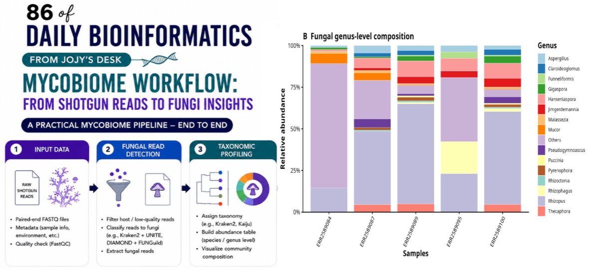
Figure 3: Genus composition
top_genera <- genus_long %>%
  group_by(Genus) %>%
  summarise(Total_Reads = sum(Reads), .groups = "drop") %>%
  arrange(desc(Total_Reads)) %>%
  slice_head(n = 15) %>%
  pull(Genus)

genus_plot <- genus_long %>%
  mutate(Genus = ifelse(Genus %in% top_genera, Genus, "Others")) %>%
  group_by(Sample, Genus) %>%
  summarise(Reads = sum(Reads), .groups = "drop") %>%
  group_by(Sample) %>%
  mutate(Relative_Abundance = Reads / sum(Reads)) %>%
  ungroup()

p3 <- ggplot(genus_plot, aes(x = Sample, y = Relative_Abundance, fill = Genus)) +
  geom_col(width = 0.85, color = "white") +
  scale_y_continuous(labels = percent) +
  theme_classic(base_size = 14) +
  labs(title = "Fungal genus composition", x = NULL, y = "Relative abundance") +
  theme(axis.text.x = element_text(angle = 45, hjust = 1))

ggsave("FigB_fungal_genus_composition.png", p3, width = 10, height = 5.5, dpi = 300)
Figure 4: Participant 1035 before and after FMT
reads_1035 <- tibble(
  Timepoint    = c("Baseline", "Week 8"),
  Fungal_Reads = c(154, 8517)
)

ggplot(reads_1035, aes(Timepoint, Fungal_Reads)) +
  geom_col(fill = "#2C7FB8") +
  geom_text(aes(label = scales::comma(Fungal_Reads)), vjust = -0.5) +
  theme_classic(base_size = 14) +
  labs(title = "Participant 1035 fungal abundance", subtitle = "Baseline vs Week 8")
154 reads at baseline. 8,517 at week 8. A ~55-fold increase following FMT. Whether this reflects donor-derived fungal engraftment, transient expansion of a resident strain, or a diet effect cannot be determined from five samples — but it is exactly the kind of signal that justifies scaling to the full 285-sample cohort.
Biological interpretation: what Kaiju can and cannot tell you
Kaiju detects DNA. DNA detection does not confirm active growth, colonization, or clinical relevance. This distinction matters especially for the environmental and dietary fungi that appear consistently in gut metagenomes:
Environmental/dietary taxa — likely transient, no colonization implied:
- Rhizopus (common bread mold)
- Hanseniaspora (fermentation yeast, found in fruit)
- Gigaspora, Claroideoglomus (soil arbuscular mycorrhizal fungi)
Host-associated taxa — more likely to reflect true gut mycobiome members:
- Candida, Pichia, Geotrichum — commensal yeasts
- Malassezia — skin-associated but detectable in stool
- Saccharomyces — common in fermented food, can persist in gut
This distinction should inform how you interpret differential abundance between FMT and placebo, or baseline and week 8. A bloom in Rhizopus may reflect a dietary change. A bloom in Candida is more likely to be biologically meaningful in an IBD context.
Scaling to 285 samples on SLURM
Download FASTQ files from ENA
# From ENA FTP file report
cut -f<fastq_ftp_col> filereport_read_run_PRJEB26357.tsv \
| tail -n +2 \
| tr ';' '\n' \
| sed 's#^#https://#' \
| xargs -n 1 -P 6 wget -c
Or using enaDataGet:
conda create -n ena_download -c bioconda -c conda-forge ena-browser-tools -y
conda activate ena_download

cut -f1 filereport_read_run_PRJEB26357.tsv | tail -n +2 > run_accessions.txt

while read RUN; do
  enaDataGet -f fastq $RUN
done < run_accessions.txt
Build a sample sheet
ls *_1.fastq.gz | sed 's/_1.fastq.gz//' > sample_ids.txt

awk 'BEGIN{OFS="\t"} {print $1, $1"_1.fastq.gz", $1"_2.fastq.gz"}' \
  sample_ids.txt > samples.tsv

wc -l samples.tsv  # should be 285
SLURM array job — one job per sample
A loop script running 285 samples sequentially would take days. A SLURM array runs them in parallel, one job per sample:
#!/bin/bash
#SBATCH --job-name=kaiju_array
#SBATCH --array=1-285%10
#SBATCH --cpus-per-task=16
#SBATCH --mem=180G
#SBATCH --time=24:00:00
#SBATCH --output=logs/kaiju_array_%A_%a.out
#SBATCH --error=logs/kaiju_array_%A_%a.err

module load kaiju/1.10.1

BASE=/scratch/jojyj/binod
RAWDIR=$BASE/raw_data
OUTDIR=$BASE/kaiju_all_results
DBDIR=/project/bcampb7/camplab/Jojy/other/kaiju

mkdir -p $OUTDIR logs

LINE=$(sed -n "${SLURM_ARRAY_TASK_ID}p" $RAWDIR/samples.tsv)
SAMPLE=$(echo $LINE | awk '{print $1}')
R1=$(echo $LINE |     awk '{print $2}')
R2=$(echo $LINE |     awk '{print $3}')

echo "Processing: $SAMPLE"

kaiju \
  -t $DBDIR/nodes.dmp \
  -f $DBDIR/kaiju_db_nr_euk.fmi \
  -i $RAWDIR/$R1 \
  -j $RAWDIR/$R2 \
  -o $OUTDIR/${SAMPLE}.out \
  -z 16 -v

kaiju-addTaxonNames \
  -t $DBDIR/nodes.dmp \
  -n $DBDIR/names.dmp \
  -i $OUTDIR/${SAMPLE}.out \
  -o $OUTDIR/${SAMPLE}.names.out \
  -r superkingdom,phylum,class,order,family,genus,species
--array=1-285%10 submits all 285 tasks but runs at most 10 simultaneously — useful for being a polite cluster user when the database loading is memory-intensive.
Submit and monitor:
sbatch run_kaiju_array.sh
squeue -u jojyj
tail -f logs/kaiju_array_JOBID_1.out
Aggregating results across all 285 samples
Phylum summary table
echo -e "Sample\tAscomycota\tMucoromycota\tBasidiomycota\tTotal_Fungal" \
  > fungal_phylum_summary_all.tsv

for f in *.names.out; do
  SAMPLE=$(basename $f .names.out)
  ASC=$(grep -c "Eukaryota; Ascomycota"    $f)
  MUC=$(grep -c "Eukaryota; Mucoromycota"  $f)
  BAS=$(grep -c "Eukaryota; Basidiomycota" $f)
  TOTAL=$((ASC+MUC+BAS))
  echo -e "${SAMPLE}\t${ASC}\t${MUC}\t${BAS}\t${TOTAL}" \
    >> fungal_phylum_summary_all.tsv
done
Genus matrix (wide format for R)
echo -e "Sample\tGenus\tReads" > fungal_genera_long_all.tsv

for f in *.names.out; do
  SAMPLE=$(basename $f .names.out)
  grep "Eukaryota; Ascomycota\|Eukaryota; Basidiomycota\|Eukaryota; Mucoromycota" $f \
  | awk -F';' '{gsub(/^ +| +$/,"",$6); if($6!="NA" && $6!="") print $6}' \
  | sort | uniq -c | sort -nr \
  | awk -v sample=$SAMPLE 'BEGIN{OFS="\t"} {print sample,$2,$1}' \
  >> fungal_genera_long_all.tsv
done
Convert to wide matrix in R:
library(tidyverse)
genus_long <- read_tsv("fungal_genera_long_all.tsv")

genus_matrix <- genus_long %>%
  pivot_wider(names_from = Genus, values_from = Reads, values_fill = 0)

write_tsv(genus_matrix, "fungal_genus_matrix_all.tsv")
Diversity analysis
Once the genus matrix is merged with metadata, standard community ecology statistics apply directly:
library(vegan)

taxa_matrix      <- genus %>% select(where(is.numeric))
sample_metadata  <- genus %>% select(any_of(c("Sample","participant","group","timepoint","response")))

# Alpha diversity
sample_metadata$Observed_Genera <- specnumber(taxa_matrix)
sample_metadata$Shannon          <- diversity(taxa_matrix, index = "shannon")

# Beta diversity
bray  <- vegdist(taxa_matrix, method = "bray")
pcoa  <- cmdscale(bray, eig = TRUE, k = 2)

# PERMANOVA
adonis2(bray ~ group + timepoint + response, data = sample_metadata, permutations = 999)
Identifying fungal-rich samples for genome recovery
Most samples will have too few fungal reads for assembly. A practical threshold for exploring fungal MAG recovery is >10,000 fungal reads; a more realistic threshold for actually obtaining a binnable fungal genome is >100,000 reads. Filter early:
fungal_rich <- phylum %>%
  arrange(desc(Total_Fungal)) %>%
  filter(Total_Fungal >= 10000)

write_tsv(fungal_rich, "fungal_rich_samples.tsv")
For samples that pass the threshold, the workflow extends into eukaryotic assembly and binning:
| Step | Recommended tools |
|---|---|
| Fungal read extraction | seqtk, BBTools |
| Assembly | MEGAHIT, metaSPAdes |
| Eukaryotic contig detection | EukRep, Tiara |
| Binning | CONCOCT, MetaBAT2 |
| Completeness assessment | BUSCO, EukCC |
| Gene annotation | funannotate, eggNOG-mapper |
Proposed next steps for the full ERP108339 cohort
The pilot validates the approach. Scaling it produces the data needed to answer the biological question: does FMT alter the gut mycobiome, and does the direction of change predict treatment response in UC?
Phase 1 — Cohort-wide mycobiome profiling: 285 metagenomes → Kaiju → genus matrix → prevalence analysis → alpha/beta diversity → identify fungal-rich samples.
Phase 2 — Clinical associations: FMT vs placebo, baseline vs week 8, treatment response stratification, candidate fungal biomarker identification. Cross-validate significant associations with Kraken2/Bracken using a eukaryote-inclusive database.
Phase 3 — Genome-resolved mycobiome: Select fungal-rich samples → extract fungal reads → assemble → EukRep/Tiara for contig filtering → bin → BUSCO/EukCC quality → annotate.
Future direction: toward genome-resolved fungal analysis
This workflow is the foundation, not the destination. Read-level classification tells you what fungi are present and in what relative proportions — but it cannot tell you anything about the functional capacity of those fungi, their genetic diversity, or whether the same Candida strain persists across timepoints or is replaced by a phylogenetically distinct isolate after FMT. Answering those questions requires genomes.
The roadmap from this pilot to genome-resolved fungal analysis has three stages, each building directly on the outputs of the last:
┌─────────────────────────────┐
│ Pilot Study                 │
│ 5 samples · Kaiju · nr_euk  │
│ Proof of concept            │
└──────────────┬──────────────┘
               │
               ▼
┌─────────────────────────────┐
│ Phase 1 · Mycobiome         │
│ Profiling                   │
│                             │
│ • Kaiju → 285 metagenomes   │
│ • Genus/phylum abundance    │
│ • Alpha & beta diversity    │
│ • Prevalence analysis       │
│ • Identify fungal-rich      │
│   samples                   │
└──────────────┬──────────────┘
               │
               ▼
┌─────────────────────────────┐
│ Phase 2 · Validation &      │
│ Clinical Associations       │
│                             │
│ • FMT vs Placebo            │
│ • Baseline vs Week 8        │
│ • Treatment response        │
│ • Candidate biomarkers      │
│ • Kraken2/Bracken cross-    │
│   validation                │
└──────────────┬──────────────┘
               │
               ▼
┌─────────────────────────────┐
│ Phase 3 · Fungal Genomics   │
│ (future work)               │
│                             │
│ • Extract fungal reads      │
│ • Assemble (MEGAHIT /       │
│   metaSPAdes)               │
│ • Eukaryotic contig ID      │
│   (EukRep, Tiara)           │
│ • MAG binning (MetaBAT2,    │
│   CONCOCT)                  │
│ • Quality: BUSCO, EukCC     │
│ • Annotation: funannotate,  │
│   eggNOG-mapper             │
└─────────────────────────────┘
Phase 3 is where this analysis becomes genuinely novel. Genome-resolved mycobiome analysis in human gut metagenomes is still a largely open field — most published studies stop at read-level classification. Recovering high-quality fungal MAGs from stool metagenomes, linking them to treatment response in IBD, and characterizing their functional gene content would represent a meaningful contribution.
Getting there requires Phase 1 and Phase 2 to work first. The fungal-rich samples that Phase 1 identifies are the input to Phase 3. The clinical associations that Phase 2 establishes determine which samples and which organisms are worth the computational investment of assembly and binning. This post covers Phase 1 in full. Phases 2 and 3 will be documented as the work develops.
This section will be updated as the genome-resolved analysis progresses.
Expected outputs
fungal_phylum_summary_all.tsv
fungal_genera_long_all.tsv
fungal_genus_matrix_all.tsv
fungal_phylum_summary_with_metadata.tsv
fungal_genus_matrix_with_metadata.tsv
fungal_alpha_diversity.tsv
fungal_genus_prevalence.tsv
fungal_rich_samples.tsv
Kaiju reference: Menzel P, Ng KL, Krogh A. “Fast and sensitive taxonomic classification for metagenomics with Kaiju.” Nature Communications 7:11257 (2016). Database: kaiju_db_nr_euk_2023-05-10. Study cohort: ERP108339 / PRJEB26357.