Genome-Resolved Metabolism: From Metabolic Potential to Co-Metabolism Networks
🧬 Genome-Resolved Metabolism: From Metabolic Potential to Co-Metabolism Networks
Hydrocarbon degradation is rarely a standalone process. In microbial genomes, it is embedded within broader metabolic frameworks that support energy conservation, redox balance, and carbon flow.
In this post, I walk through a complete workflow for analyzing metabolic potential, co-energy metabolism, and co-metabolism networks in hydrocarbon-degrading MAGs—starting from marker gene detection and ending with bipartite network visualization.
This workflow is directly applicable to metagenome-assembled genomes (MAGs) and is essential for functional ecology, biogeochemistry, and multi-omics studies.
🎯 What Are We Trying to Answer?
Three related but distinct questions drive this analysis:
1. Metabolic Potential
What other metabolic capabilities are encoded in MAGs that contain hydrocarbon degradation genes?
This asks: What is possible?
2. Co-Energy Metabolism
Which energy generation and conservation pathways co-occur with hydrocarbon degradation?
This asks: How is degradation energetically supported?
3. Co-Metabolism
Which metabolic pathways are actively expressed together within the same genome?
This asks: What is actually used together?
These questions require different analytical approaches:
| Question | Data Type | Visualization |
|---|---|---|
| Metabolic potential | Gene presence/absence | Binary heatmap |
| Co-energy | Gene presence/absence | Binary heatmap |
| Co-metabolism | Gene expression | Scaled heatmap + Network |
🧪 Part 1: Identifying Hydrocarbon-Degrading MAGs
We first subset MAGs that contain at least one hydrocarbon degradation gene (e.g., alkB, bssA, assA, or DSR-associated alkyl pathways).
These MAGs form the foundation for all downstream analyses.
🔍 Part 2: Assessing Metabolic Flexibility
Metabolic flexibility describes the capacity of a genome to encode and potentially utilize multiple metabolic pathways simultaneously, allowing organisms to adapt to fluctuating environmental conditions and substrate availability.
🧬 Step-by-Step Workflow
Step 1: Download Metabolic Marker Gene Sets
We downloaded curated metabolic marker protein sequences from the Greening Lab Metabolic Marker Database, which includes high-confidence markers for:
- Respiration (aerobic and anaerobic)
- Sulfur cycling (oxidation and reduction)
- Nitrogen cycling (fixation, nitrification, denitrification)
- Carbon fixation (CBB cycle, rTCA, Wood-Ljungdahl)
- Phototrophy (photosystems, reaction centers)
Step 2: Build a DIAMOND Database
The downloaded marker protein sequences were combined into a single FASTA file and formatted as a DIAMOND database:
diamond makedb \
  --in metabolic_markers.faa \
  --db metabolic_markers \
  --threads 16
Step 3: Predict Proteins from MAGs
Protein-coding genes were predicted from MAGs using Prodigal:
prodigal \
  -i MAGs.fna \
  -a MAGs_proteins.faa \
  -p meta \
  -q
Step 4: Search MAG Proteins Against Metabolic Markers
Predicted proteins from each MAG were queried against the metabolic marker database using DIAMOND BLASTp:
diamond blastp \
  --query MAGs_proteins.faa \
  --db metabolic_markers \
  --out metabolic_hits.tsv \
  --outfmt 6 qseqid sseqid pident length evalue bitscore \
  --evalue 1e-5 \
  --max-target-seqs 1 \
  --threads 16
Step 5: Summarize Metabolic Marker Presence
DIAMOND hits were parsed to generate a MAG × metabolic marker table, summarizing:
- Presence/absence of each metabolic marker
- Number of marker genes per metabolic process per MAG
# Parse DIAMOND output
awk '{print $1,$2}' metabolic_hits.tsv | \
  sed 's/_.*//' | \
  sort -u > MAG_marker_presence.tsv
This table forms the basis for downstream analyses of metabolic potential and metabolic flexibility.
📊 Part 3: Visualizing Metabolic Potential
What Does This Show?
For each hydrocarbon-degrading MAG, we determine whether it encodes key marker genes for:
- Respiration (terminal oxidases, electron transport)
- Sulfur cycling (sulfur oxidation, sulfate reduction)
- Nitrogen cycling (nitrogen fixation, denitrification)
- Carbon fixation (autotrophic pathways)
- Phototrophy (light harvesting, energy conversion)
This is genomic potential—not expression.
📁 Input Format (Example)
| MAG | Order | Gene | Process |
|---|---|---|---|
| MAG_01 | Burkholderiales | AtpA | Respiration |
| MAG_01 | Burkholderiales | Sqr | Sulfur cycle |
| MAG_02 | Pseudomonadales | NarG | Nitrogen cycle |
| MAG_02 | Pseudomonadales | RuBisCO | Carbon fixation |
📊 Presence–Absence Heatmap in R
library(pheatmap)
library(dplyr)
library(tidyr)

# Read metabolic potential data
metabolic_df <- read.csv("MAG_metabolic_markers.csv")

# Create binary matrix: 1 = gene present, 0 = absent
pot_mat <- metabolic_df %>%
  mutate(present = 1) %>%
  pivot_wider(
    names_from = MAG,
    values_from = present,
    values_fill = 0
  )

mat <- as.matrix(pot_mat[, -1])
rownames(mat) <- pot_mat$Gene

# Create heatmap
pheatmap(
  mat,
  color = c("white", "steelblue"),
  cluster_rows = FALSE,
  cluster_cols = TRUE,
  legend = TRUE,
  show_rownames = TRUE,
  show_colnames = TRUE,
  fontsize_row = 8,
  fontsize_col = 10,
  main = "Metabolic Potential of Hydrocarbon-Degrading MAGs",
  cellwidth = 20,
  cellheight = 12
)
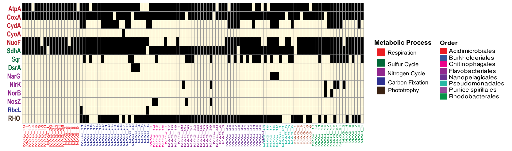
🧠 Interpretation
Key findings:
✅ Respiration genes are widespread across most MAGs
✅ Sulfur and nitrogen cycling genes are patchy and taxon-specific
✅ Carbon fixation and phototrophy are restricted to a subset of genomes
Key insight:
Hydrocarbon degradation occurs within metabolically diverse genomic backgrounds, not a single conserved metabolic blueprint.
⚡ Part 4: Co-Energy Metabolism Analysis
What Is Co-Energy?
Co-energy examines which energy generation and conservation pathways co-occur with hydrocarbon degradation in the same genome.
Key pathways analyzed:
- Aerobic respiration (cytochrome c oxidases)
- Anaerobic respiration (nitrate, sulfate, Fe(III) reduction)
- Fermentation (substrate-level phosphorylation)
- ATP synthase (energy conservation)
📊 Co-Energy Heatmap
# Subset to energy-related markers only
energy_genes <- c(
  "coxA", "coxB", "cydA",           # Aerobic respiration
  "narG", "napA", "nirK", "nosZ",   # Denitrification
  "dsrA", "aprA",                   # Sulfate reduction
  "atpA", "atpD",                   # ATP synthase
  "pdhA", "ackA", "pta"             # Fermentation
)

energy_mat <- mat[rownames(mat) %in% energy_genes, ]

pheatmap(
  energy_mat,
  color = c("white", "#d95f02"),
  cluster_rows = TRUE,
  cluster_cols = TRUE,
  main = "Co-Energy: Energy Pathways in HC-Degrading MAGs"
)
Key insight:
Energy metabolism is heterogeneous across hydrocarbon-degrading taxa, suggesting niche partitioning along redox gradients.
🔥 Part 5: From Potential to Co-Metabolism
Metabolic potential tells us what is possible.
Co-metabolism asks what is used together.
We now shift from presence/absence to gene expression data.
Focus: Five Core Metabolic Categories
- Hydrocarbon degradation — Primary substrate utilization
- C1 metabolism — Single-carbon compound cycling
- Complex carbon degradation — Polymeric substrate breakdown
- Fermentation — Anaerobic energy generation
- Central carbon metabolism — Glycolysis, TCA cycle, pentose phosphate pathway
📥 Part 6: Prepare Expression Data
Data Structure
Expression data should contain:
- MAG identifiers (e.g., Burkholderiales_MAG_10)
- Gene names (e.g., enolase, citrate synthase)
- Metabolic categories (e.g., Central carbon metabolism)
- Sample-specific counts (raw counts or TPM values)
R Code for Data Preparation
library(readxl)
library(dplyr)
library(stringr)

# Load expression data
df <- read_excel("Burk_gene_summed_filtered.xlsx")

# Clean column names
names(df) <- tolower(gsub(" ", "_", names(df)))

# Preserve raw categories for QC
df$category_raw <- df$category

# Define metadata vs count columns
meta_cols <- c("mags", "order", "gene.name", "category", "category_raw", "pathway")
count_cols <- setdiff(names(df), meta_cols)

# Convert counts to numeric
df[count_cols] <- lapply(df[count_cols], as.numeric)

# Check for NA values
if (any(is.na(df[count_cols]))) {
  stop("❌ NA values found in count columns — check input file")
}
Critical QC Step: Standardize Categories
# Normalize category names
df$category <- df$category_raw %>%
  str_trim() %>%
  str_to_lower() %>%
  str_replace_all("\\s+", " ")

# Recode to standard names
df$category <- case_when(
  str_detect(df$category, "hydrocarbon") ~ "Hydrocarbon degradation",
  str_detect(df$category, "^c1")         ~ "C1 metabolism",
  str_detect(df$category, "complex")     ~ "Complex carbon degradation",
  str_detect(df$category, "ferment")     ~ "Fermentation",
  str_detect(df$category, "central")     ~ "Central carbon metabolism",
  TRUE                                   ~ NA_character_
)

# Remove uncategorized genes
cat("\n📊 Category distribution BEFORE removing NAs:\n")
print(table(df$category, useNA = "ifany"))

df <- df %>% filter(!is.na(category))

cat("\n✅ Category distribution AFTER removing NAs:\n")
print(table(df$category, useNA = "ifany"))
Why this matters:
Inconsistent category names (e.g., “Hydrocarbon Degradation” vs “hydrocarbon degradation”) will create duplicate categories and an “NA” group in your heatmap legend.
Create Factor Levels
df$category <- factor(
  df$category,
  levels = c(
    "Hydrocarbon degradation",
    "C1 metabolism",
    "Complex carbon degradation",
    "Fermentation",
    "Central carbon metabolism"
  )
)
Log2 Transform Expression Data
# Create expression matrix
mat <- as.matrix(df[, count_cols])

# Create unique gene IDs
df$gene_id <- make.unique(
  paste(df$mags, df$category, df$gene.name, sep = "|")
)
rownames(mat) <- df$gene_id

# Log2 transform: stabilizes variance, makes patterns visible
mat_log <- log2(mat + 1)
Why log2(x + 1)?
- Stabilizes variance across expression ranges
- Makes patterns more visible
- The “+1” prevents log(0) = -∞ (pseudocount)
- Standard for RNA-seq and metatranscriptomics
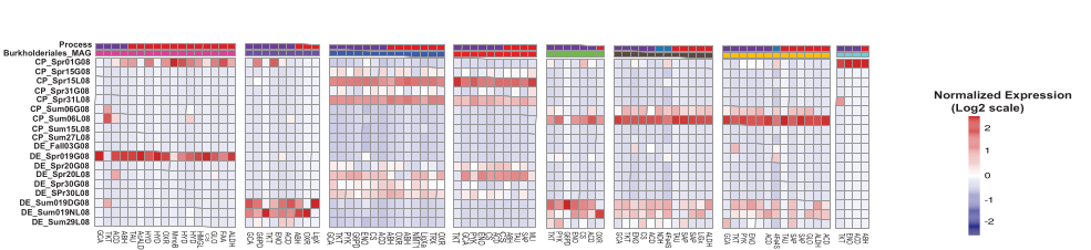
🎨 Part 7: Co-Metabolism Heatmap (Row-Scaled)
Row Scaling: The Critical Decision
Row scaling converts expression values to Z-scores for each gene:
Z-score = (value - gene_mean) / gene_standard_deviation
Why use row scaling?
- ✅ Genes have vastly different expression levels
- ✅ Highlights relative patterns within each gene
- ✅ Makes all genes visually comparable
- ✅ Standard for gene expression publications
Color interpretation:
- Blue (negative): Gene is expressed below its own average
- White (zero): Gene is at its average expression
- Red (positive): Gene is expressed above its own average
Prepare Row Annotations
# Extract MAG number
df$mag_num <- as.numeric(
  str_extract(tolower(df$mags), "(?<=_mag_)\\d+")
)

# Remove rows with unextractable MAG numbers
if (any(is.na(df$mag_num))) {
  df <- df %>% filter(!is.na(mag_num))
  mat_log <- mat_log[rownames(mat_log) %in% df$gene_id, ]
}

# Order by MAG, then category
row_order <- order(df$mag_num, df$category)
heat_sorted <- mat_log[row_order, ]
df_sorted <- df[row_order, ]

# Create annotation data frame
ann_row <- data.frame(
  MAG = factor(df_sorted$mag_num),
  Category = df_sorted$category
)
rownames(ann_row) <- rownames(heat_sorted)
Define Color Schemes
ann_colors <- list(
  MAG = setNames(
    rainbow(length(unique(df_sorted$mag_num))),
    sort(unique(df_sorted$mag_num))
  ),
  Category = c(
    "Hydrocarbon degradation" = "#e31a1c",
    "C1 metabolism" = "#1f78b4",
    "Complex carbon degradation" = "#33a02c",
    "Fermentation" = "#ff7f00",
    "Central carbon metabolism" = "#6a3d9a"
  )
)
Clean Sample Labels
pretty_labels <- toupper(colnames(heat_sorted))
pretty_labels <- gsub("_", " ", pretty_labels)
gene_labels <- df_sorted$gene.name
Generate the Heatmap
library(pheatmap)

pheatmap(
  heat_sorted,
  scale = "row",                    # Z-score normalization
  cluster_rows = FALSE,             # Preserve MAG/category order
  cluster_cols = FALSE,             # Preserve sample order
  show_rownames = TRUE,             # Display gene names
  labels_row = gene_labels,
  labels_col = pretty_labels,
  angle_col = 45,
  fontsize_row = 3,                 # Small font for many genes
  fontsize_col = 8,
  gaps_row = cumsum(table(df_sorted$mag_num)),  # Visual gaps between MAGs
  annotation_row = ann_row,
  annotation_colors = ann_colors,
  color = colorRampPalette(c("navy", "white", "firebrick3"))(100),
  legend = TRUE,
  legend_breaks = seq(-2, 2, 1),
  legend_labels = c("-2", "-1", "0", "1", "2"),
  main = "Co-Metabolism Gene Expression by MAG",
  fontsize = 10
)
📖 Legend Interpretation
Your legend should read:
Abundance
(Log 2+1)
Z-score
Values: -2, -1, 0, 1, 2
These represent standard deviations from the mean, NOT:
- ❌ Raw counts
- ❌ Fold-changes
- ❌ Absolute abundance
🌐 Part 8: Build a Co-Metabolism Network
Heatmaps show patterns.
Networks reveal structure.
We now convert the expression matrix into a bipartite network where:
- Nodes = MAGs and metabolic categories
- Edges = Average co-expression strength between MAG and category
Step 1: Aggregate Expression by MAG × Category
library(igraph)
library(ggraph)
library(tidyr)

# Calculate mean expression per MAG-category pair
agg_df <- df_sorted %>%
  rowwise() %>%
  mutate(mean_expr = mean(c_across(all_of(count_cols)))) %>%
  ungroup() %>%
  group_by(MAG = mags, Category = category) %>%
  summarise(mean_expr = mean(mean_expr), .groups = "drop")

# Normalize edge weights
agg_df$weight <- agg_df$mean_expr / max(agg_df$mean_expr)
Step 2: Create Bipartite Graph
# Create edge list
edges <- data.frame(
  from = agg_df$MAG,
  to = agg_df$Category,
  weight = agg_df$weight
)

# Build graph
g <- graph_from_data_frame(edges, directed = FALSE)

# Assign node types
V(g)$type <- ifelse(V(g)$name %in% unique(agg_df$MAG), "MAG", "Category")

# Calculate node degree
V(g)$degree <- degree(g)
Step 3: Visualize the Network
set.seed(42)  # For reproducibility

ggraph(g, layout = "fr") +
  geom_edge_link(
    aes(width = weight, alpha = weight),
    color = "grey50"
  ) +
  geom_node_point(
    aes(size = degree, color = type),
    alpha = 0.8
  ) +
  geom_node_text(
    aes(label = name),
    repel = TRUE,
    size = 3,
    fontface = "bold"
  ) +
  scale_edge_width(range = c(0.2, 2), guide = "none") +
  scale_edge_alpha(range = c(0.3, 0.9), guide = "none") +
  scale_size(range = c(4, 16), name = "Degree") +
  scale_color_manual(
    values = c("MAG" = "#377eb8", "Category" = "#e41a1c"),
    name = "Node Type"
  ) +
  theme_void() +
  theme(
    legend.position = "right",
    plot.title = element_text(hjust = 0.5, size = 14, face = "bold")
  ) +
  ggtitle("MAG–Category Co-Metabolism Network")
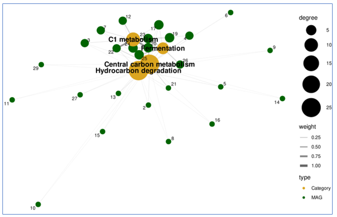
🧠 Part 9: How to Read the Network
Node Interpretation
Category nodes (red):
- Metabolic hubs
- Node size = number of MAGs connected
- Larger nodes = more broadly used pathways
MAG nodes (blue):
- Individual genomes
- Node size = number of pathways engaged
- Larger nodes = more metabolically integrated genomes
Edge Interpretation
Edge thickness:
- Represents strength of co-metabolic activity
- Thicker edges = stronger co-expression
- Thinner edges = weaker or conditional usage
🧪 Why This Matters
This workflow demonstrates that:
1. Hydrocarbon Degradation Is Metabolically Embedded
- Not an isolated function
- Requires coordinated energy metabolism
- Supported by central carbon pathways
2. Taxa Differ in Metabolic Integration
- Pseudomonadales: high integration, constitutive expression
- Burkholderiales: flexible, condition-responsive expression
- Reflects different ecological strategies
3. Co-Metabolism Networks Reveal Hidden Structure
- Heatmaps show expression patterns
- Networks reveal metabolic integration architecture
- Essential for understanding microbial community function
🆚 When to Use Each Visualization
| Visualization | Best For | Data Type | Interpretation |
|---|---|---|---|
| Binary heatmap | Metabolic potential | Presence/absence | What is possible? |
| Binary heatmap | Co-energy | Presence/absence | Which energy pathways co-occur? |
| Scaled heatmap | Co-metabolism | Gene expression | What is used together? |
| Network | Metabolic integration | Aggregated expression | How are pathways structurally connected? |
📌 Key Takeaways
✅ Separate metabolic potential from co-metabolism
- Potential = what’s encoded (genomic)
- Co-metabolism = what’s expressed (functional)
✅ Use row scaling (Z-scores) for expression heatmaps
- Standard for gene expression analysis
- Enables comparison across genes with different expression ranges
✅ Networks reveal metabolic integration structure
- Complements heatmaps
- Shows hub pathways and specialist taxa
✅ Co-metabolism differs strongly across taxa
- Not all hydrocarbon degraders are metabolically equivalent
- Functional diversity emerges from co-metabolic strategies
✅ Genome-resolved approaches are essential
- Bulk metagenomics/metatranscriptomics miss this complexity
- MAG-level resolution reveals individual strategies
💬 Questions?
Drop a comment below! I’m happy to help troubleshoot or discuss adaptations for different systems.