Day 5: Substrate Uptake & Utilization in Size-Fractionated Estuarine Microbiomes
🧬 Day 5: Substrate Uptake & Utilization in Size-Fractionated Estuarine Microbiomes
From gene catalogs to carbon currency
Marine environments are heterogeneous, largely due to suspended particles that create metabolically distinct niches compared to free-living waters. While taxonomic partitioning between free-living (FL) and particle-attached (PA) bacteria is well documented, how this separation shapes substrate utilization and carbon flow remains less clear.
In this post, I move beyond taxonomy and into mechanism.
I trace substrate utilization from:
- Gene prediction
- Functional annotation (CAZymes, ABC transporters, TonB-dependent transporters)
- Mapping metagenomes & metatranscriptomes
- Functional filtering
- Heatmap visualization
This is the functional backbone of size-fractionated microbiome ecology.
🔬 Step 1: Build a Concatenated Gene Catalog
After assembling and binning MAGs, genes were predicted using Prodigal:
# Gene prediction
prodigal -i MAG.fasta -a MAG.faa -d MAG.fna -p meta
Please see batch_scripts in 5th Day repo
All predicted genes were then concatenated into a unified reference:
cat *.faa > all_genes.faa
cat *.fna > all_genes.fna
Why concatenate?
● Ensures consistent mapping reference
● Allows competitive read assignment
● Avoids sample-specific gene catalogs
● Simplifies downstream quantification
This unified gene catalog becomes the reference for both metagenomic (MG) and metatranscriptomic (MT) mapping.
Step 2: Dereplicate the concatenated gene catalog with CD-HIT-EST
Before building the Bowtie2 index and mapping reads, I dereplicated the concatenated gene FASTA to remove redundant sequences and create a non-redundant reference. This reduces ambiguous multi-mapping and makes downstream abundance estimates more stable.
Run CD-HIT-EST (example: 90% identity)
module load cd-hit

IN=all_genes_concat.fa
OUT=MG_gene_catalog90

cd-hit-est \
  -i "$IN" \
  -o "$OUT" \
  -c 0.90 \
  -n 8 \
  -aS 0.80 \
  -G 0 \
  -T 24 \
  -M 0 \
  > "${OUT}.cdhit.log" 2>&1
Output files
● MG_gene_catalog90 → dereplicated gene FASTA (use this for indexing/mapping)
● MG_gene_catalog90.clstr → clustering report (which sequences were grouped)
Tip: If you want stricter dereplication (more collapsing), increase -c (e.g., 0.95). If you want to keep more diversity, reduce it slightly (e.g., 0.85–0.90 depending on your goal).
🧪 Step 3: Functional Annotation
This custom annotation was used to create a gff file for mapping gene ids with its corresponding gene name.
🧬 3A. CAZymes (dbCAN)
Carbohydrate-active enzymes were identified using dbCAN:
run_dbcan.py all_genes.faa protein --out_dir dbcan_out
Hits were filtered based on:
● HMMER E-value thresholds
● Alignment coverage
I extracted:
All gene ids and thier gene class including GH (glycoside hydrolases); AA (auxiliary activity enzymes),CBM (carbohydrate-binding modules), etc.
🚪 2B. Transporters
- ABC transporters were annotated via:
● KEGG orthology mapping
● TCDB classification
● Custom HMM searches
Focused on:
● 3.A.1.x families
● Sugar and oligosaccharide importers
- TonB-Dependent Transporters (TBDTs)
Outer membrane TonB-dependent transporters were identified using HMM searches:
🎯 Step 3: Mapping Reads Back to Genes
Metagenomes and Metatranscriptomes All metagenomes and metatranscriptomes were mapped to a index file which generated using the concatenated fasta using bowtie
module load bowtie2
module load samtools
# Build index from dereplicated gene catalog
bowtie2-build MG_gene_catalog90 MG_gene_catalog90_index
# Example paired-end MG mapping
bowtie2 \
  -x MG_gene_catalog90_index \
  -1 sample_MG_R1.fastq.gz \
  -2 sample_MG_R2.fastq.gz \
  --very-sensitive \
  -p 24 \
| samtools sort -@ 24 -o sample_MG.bam

samtools index sample_MG.bam

# Example paired-end MT mapping
bowtie2 \
  -x MG_gene_catalog90_index \
  -1 sample_MT_R1.fastq.gz \
  -2 sample_MT_R2.fastq.gz \
  --very-sensitive \
  -p 24 \
| samtools sort -@ 24 -o sample_MT.bam

samtools index sample_MT.bam
The resulting BAM files were used to generate gene-level count matrices for downstream functional filtering and heatmap analysis.
🧮 Step 4: Filtering Functional Groups inPython
Once counts were generated, functional subsets were extracted using custom python scripts. The files were really big so I run it on HPC. The final files were exported to the local desktop and
were aggregated by:
●MAG
● Functional category
● Bay
● Season
● Size fraction
Using custom scripts in Pandas, below is an example with TonB expression data:
import pandas as pd

# Load the Excel files
feature_table = pd.read_excel('/home/jojy-john/Jojy_Research_Sync/Fl_vs_Pa/substrte_uptake_finalfiles_feb19/all_files/final/MT_TonB_averaged.xlsx')
annotation = pd.read_excel('/home/jojy-john/Jojy_Research_Sync/Fl_vs_Pa/substrte_uptake_finalfiles_feb19/all_files/TonB_refrence.xlsx')

# Strip column names
feature_table.columns = feature_table.columns.str.strip()
annotation.columns = annotation.columns.str.strip()

# --------------------------------------------------
# CLEAN THE ID COLUMN (Very Important)
# --------------------------------------------------

# Convert to string (important if Excel treated them as numbers)
feature_table['id'] = feature_table['id'].astype(str).str.strip()
annotation['id'] = annotation['id'].astype(str).str.strip()

# Optional: remove ALL spaces inside IDs (if needed)
# feature_table['id'] = feature_table['id'].str.replace(" ", "")
# annotation['id'] = annotation['id'].str.replace(" ", "")

# --------------------------------------------------
# Merge
# --------------------------------------------------
merged = pd.merge(feature_table, annotation, on='id', how='left', indicator=True)

# Matching rows (present in both)
matched = merged[merged['_merge'] == 'both']
matched.to_excel('/home/jojy-john/Jojy_Research_Sync/Fl_vs_Pa/substrte_uptake_finalfiles_feb19/all_files/final/MT_TonB_mapped.xlsx', index=False)

print("Merging complete. Matching file saved.")
What I did here?
● To link TonB expression values to their functional annotations, I merged the averaged metatranscriptomic count table with a curated TonB reference file using a shared gene id
● First, both Excel files were loaded with pandas and column names were cleaned to remove hidden spaces. Because Excel sometimes converts IDs to numeric format, the id column in both tables was explicitly converted to string and stripped of extra whitespace to ensure exact matching.
● A left join (how=’left’) was then performed to merge expression values with annotation metadata. Only rows present in both tables were retained as matched genes, and the final merged dataset was exported for downstream analysis.
● This step ensures that expression values are accurately linked to their functional classifications before filtering and visualization.
After mapping TonB genes to their functional annotations, I summarized expression at the gene family (or class) level. Since multiple genes can belong to the same TonB family, raw gene-level counts were grouped by the family column and summed across all samples.
import pandas as pd

# Input Excel file
infile = "/home/jojy-john/Jojy_Research_Sync/Fl_vs_Pa/substrte_uptake_finalfiles_feb19/all_files/final/MT_TonB_mapped.xlsx"

# Output file
outfile = "/home/jojy-john/Jojy_Research_Sync/Fl_vs_Pa/substrte_uptake_finalfiles_feb19/all_files/final/MT_TonB_final.xlsx.xlsx"

# Read Excel
df = pd.read_excel(infile)

# Group by 2nd column
df_sum = df.groupby(df.columns[1], as_index=False).sum(numeric_only=True)

# Save back to Excel
df_sum.to_excel(outfile, index=False)

print("Done.")
This final file was used for remaining downstream analysis including generating heatmaps.
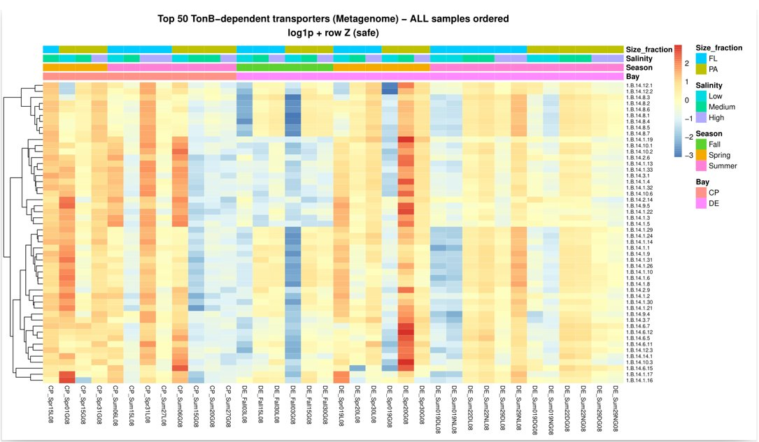
📊 Step 5: Normalization & Heatmap Visualization
● Raw counts were log-transformed: ● To highlight relative patterns across samples, row-wise Z-score scaling was applied: ● Heatmaps were generated using Pheatmap
please see TonB_heatmap.R in 5th Day repo
🌱 What Did I Observe?
● GH13 glycoside hydrolases dominated across bays.
● FL communities were enriched in oxidative AA enzymes.
● Chesapeake Bay showed salinity-driven transcriptional gating.
● Delaware Bay exhibited bloom-associated coordination.
● ABC sugar importers were consistently abundant.
● TonB transporters peaked in PA communities during bloom events.
● These patterns suggest that extracellular degradation and intracellular uptake are tightly coordinated during productive periods.
🧠 Key Takeaways
● Size fractionation structures functional strategy.
● CAZymes and transporters operate as a coordinated system.
● Bloom dynamics drive synchronized degradation and uptake.
● Oligosaccharides act as a central carbon currency in estuarine systems.
🌊 Closing Thoughts
● Size-fractionated microbiome studies reveal more than community composition — they uncover how carbon moves through ecosystems.
● By linking extracellular degradation to transporter-mediated uptake, we gain insight into the metabolic economics shaping estuarine microbiomes.
The Abstarct is submitted to ISME 20 in Auckland, New Zealand on 16-21 August 2026
All codes are availble in 5th Day repo
Previous Days of this same series can be found as follows : 📖 Day 1: From Raw Reads to Clean Data
📖 Day 2: Kaiju Classification and Extraction of Bacterial & Archaeal Reads
📖 Day 3: Species-Level Profiling with mOTUs
📖 Day 4: Gene Catalog Construction & Functional Annotation
All codes are availble in 5th Day repo