Building a Custom GTDBtk Database for HUMAnN3 — A Gene Catalogue Approach for Environmental Metagenomics
Building a custom GTDBtk database for HUMAnN3 — a gene catalogue approach for environmental metagenomics
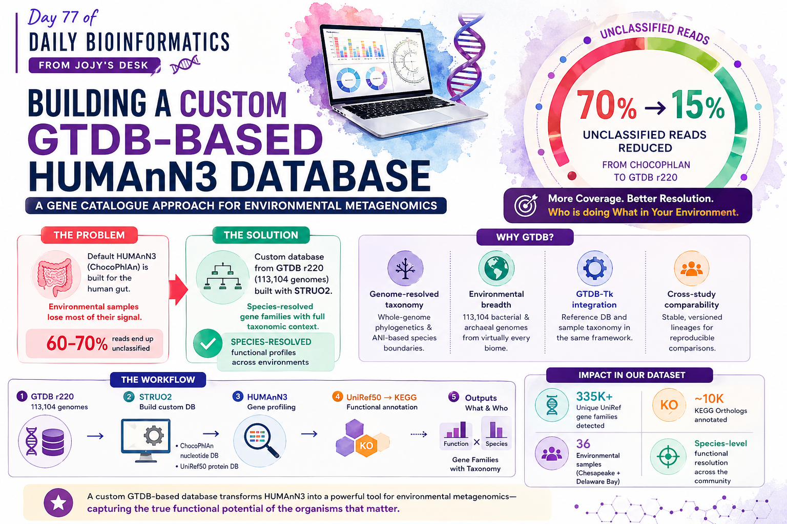
🧬 𝐷𝑎𝑦 77 𝑜𝑓 𝐷𝑎𝑖𝑙𝑦 𝐵𝑖𝑜𝑖𝑛𝑓𝑜𝑟𝑚𝑎𝑡𝑖𝑐𝑠 𝑓𝑟𝑜𝑚 𝐽𝑜𝑗𝑦’𝑠 desk
If you work with environmental microbial communities — estuaries, soils, marine systems — you have probably run into the same frustration: HUMAnN3’s default ChocoPhlAn database was built for the human gut. Use it on an estuary sample and you will miss most of the community.
The coverage problem is concrete. In our Chesapeake and Delaware Bay metagenomes, HUMAnN3 with ChocoPhlAn left the majority of reads unclassified at the species level and relegated them to an “unmapped” or “unintegrated” catch-all. Using a custom database built from GTDB release 220 (113,104 bacterial and archaeal genomes), we went from fragmented community profiles to species-resolved gene families covering the organisms that actually matter in that environment.
A custom database also gives you something the default workflow cannot: full taxonomic context linked to GTDB phylogeny. Every gene family output by HUMAnN3 carries a species label traceable back to a GTDB lineage, enabling downstream analyses that require knowing who is doing what.
Why GTDB over SILVA or NCBI for this purpose?
Before diving into the workflow, it is worth explaining the choice of GTDB (Genome Taxonomy Database) as the reference framework.
Genome-resolved taxonomy: GTDB is built from whole-genome phylogenetics, not marker genes. Species boundaries are based on average nucleotide identity (ANI), making them more reproducible and less subject to historical naming inconsistencies.
Environmental breadth: GTDB r220 includes 113,104 bacterial and archaeal genomes spanning virtually every biome sequenced to date — far broader representation of environmental taxa than gut-focused catalogues.
GTDB-Tk integration: GTDB-Tk annotates query genomes and assigns them to the GTDB tree, so your reference database and your sample taxonomy live in the same coordinate system.
Cross-study comparability: GTDB lineage labels are stable and versioned, making your gene catalogue directly comparable to other GTDB-based studies.
Step 1: Building the HUMAnN3-friendly database with STRUO2
STRUO2 (Streamlined Update of Omics Reference material) is a Snakemake pipeline that takes a genome collection and produces exactly the files HUMAnN3 needs: a custom ChocoPhlAn-equivalent nucleotide database and a DIAMOND-formatted protein database with UniRef50 annotations.
What STRUO2 needs
| Input | Description |
|---|---|
| Genome directory | GTDB genomes in GCA/XXX/XXX/XXX/ structure |
genome_metadata.tsv | Columns: genome name, species, NCBI taxid |
genome_reps_filt_annot.tsv.gz | Gene → UniRef50 ID mapping from GTDB-Tk/eggNOG |
Running STRUO2
# Configure in config.yaml:
# genomes_dir: /path/to/gtdb_release220/genomes/
# genome_table: genome_metadata.tsv
# annot_file: genome_reps_filt_annot.tsv.gz
# output_dir: /path/to/gtdb_for_humann3/

snakemake --snakefile Snakefile \
          --configfile config.yaml \
          --cores 64 \
          --use-conda
Key outputs
gtdb_for_humann3/
├── uniref50/
│   └── uniref50_201901b.dmnd      # DIAMOND protein database
├── chocophlan/
│   └── *.ffn.gz                   # Nucleotide marker genes
└── genome_reps_filt_annot.tsv.gz  # Gene annotation table
The uniref50/ directory is what you pass to HUMAnN3’s --protein-database flag. For our GTDB r220 build this produced ~696,000 unique annotated genes.
Step 2: Running HUMAnN3 with the custom database
With the custom database in hand, HUMAnN3 runs identically to a standard analysis — you simply point it to your database directory.
humann \
  --input sample_R1_R2_cat.fastq \
  --output humann_output/ \
  --threads 32 \
  --nucleotide-database /path/to/gtdb_for_humann3/chocophlan/ \
  --protein-database /path/to/gtdb_for_humann3/uniref50/uniref50_201901b.dmnd \
  --taxonomic-profile sample_metaphlan.tsv   # optional: speeds up nucleotide step
A few practical notes: concatenate paired-end reads before passing them in (cat R1.fastq R2.fastq > merged.fastq). If you have a MetaPhlAn4 profile generated against GTDB already, pass it with --taxonomic-profile to skip the nucleotide search and save time. For large sample sets, wrap this in a SLURM array — each sample is fully independent.
In our 36-sample dataset (Chesapeake + Delaware Bay metagenomes) this detected 335,121 unique UniRef gene families with species stratification.
Step 3: Understanding the HUMAnN3 outputs
Each sample produces three files.
*_genefamilies.tsv — the core output
Rows are gene families (UniRef50 IDs), values are RPK (reads per kilobase). Critically, each UniRef entry is broken into species-stratified rows:
# Gene Family                               Sample_Abundance
UniRef50_A0A000|unclassified                142.3
UniRef50_A0A000|s__Marinobacter_adhaerens    98.7
UniRef50_A0A000|s__Alteromonas_macleodii     43.6
The |unclassified row captures reads mapping to that gene family but not assignable to a species in your database. With a gut database on an estuary sample this fraction is huge (>60%); with a GTDB-based custom database it drops dramatically.
*_pathabundance.tsv
MetaCyc pathway abundances summed across contributing gene families, also species-stratified. Useful for rapid pathway-level summaries and comparing metabolic potential across samples.
*_pathcoverage.tsv
The fraction of genes detected per pathway (0–1). Coverage < 1 means a pathway is only partially present; coverage = 1 means every expected gene was detected. Useful for filtering complete vs incomplete pathways before downstream analysis.
Merging and normalizing across samples
# Merge all samples into a single table
humann_join_tables \
  --input humann_output/ \
  --output merged_genefamilies.tsv \
  --file_name genefamilies

# Normalize to copies per million
humann_renorm_table \
  --input merged_genefamilies.tsv \
  --output merged_genefamilies_cpm.tsv \
  --units cpm
Normalization is essential before any cross-sample comparison — raw RPK values are confounded by sequencing depth.
Step 4: Mapping UniRef50 to KEGG Orthology
HUMAnN3 outputs UniRef50 IDs — functional sequence clusters. For ecological interpretation, it is more useful to work at the KEGG Orthology (KO) level. KOs group proteins by biological function and carry pathway and module context.
humann_regroup_table \
  --input merged_genefamilies_cpm.tsv \
  --output merged_KOs.tsv \
  --groups uniref50_ko
In our dataset this reduced 335,121 UniRef gene families to roughly 5,000–15,000 biologically meaningful KO groups — a ~95% reduction in matrix size with no meaningful loss of ecological signal. The KO table is faster to compute, easier to interpret, and directly usable in pathway enrichment analyses.
Step 5: Building the genome × KO trait table
For genome-resolved analyses — functional redundancy, niche differentiation — you need to link HUMAnN3’s species-stratified outputs back to individual reference genomes and produce a binary genome × KO trait matrix.
library(tidyverse)

ko_table <- read_tsv("merged_KOs.tsv")

# Keep only species-stratified rows, drop unclassified
ko_species <- ko_table %>%
  filter(str_detect(`# Gene Family`, "\\|"),
         !str_detect(`# Gene Family`, "unclassified")) %>%
  separate(`# Gene Family`, into = c("KO", "species"), sep = "\\|")

# Build binary presence/absence matrix
trait_matrix <- ko_species %>%
  group_by(species, KO) %>%
  summarise(present = 1, .groups = "drop") %>%
  pivot_wider(names_from  = KO,
              values_from = present,
              values_fill = 0)
This matrix — 1,000 genomes × ~10,000 KOs in our case — is the gene catalogue. Each row is a reference genome, each column a function, and the binary values encode functional potential.
Taxonomy conjugation
Because your HUMAnN3 species labels are GTDB lineages, you can seamlessly combine functional profiles with phylogenetic trees from GTDB-Tk, comparative genomics databases, and diversity metrics that require a consistent taxonomy. This cross-linking is not possible when your functional profiles use one taxonomy (MetaPhlAn/SILVA) and your genomic analyses use another (GTDB).
Performance comparison: custom GTDB vs. default ChocoPhlAn
| Metric | Default ChocoPhlAn | Custom GTDB DB |
|---|---|---|
| Unclassified reads | ~60–70% in environmental samples | ~15–25% |
| Species detected | Gut-biased, low diversity | Environment-matched |
| Taxonomy framework | MetaPhlAn/SILVA | GTDB (genome-resolved) |
| KEGG annotation | Via HUMAnN3 utility | Via HUMAnN3 utility |
| Cross-study comparability | Limited (gut studies) | High (GTDB-based) |
| Database build time | N/A (pre-built) | ~24–48 hrs for GTDB r220 |
The upfront cost of building the custom database — one-time, around 48 hours on 64 cores — is dwarfed by the gains in classification rate and ecological interpretability.
Summary
Building a custom GTDBtk-based database for HUMAnN3 is not just a technical improvement — it is the correct approach for environmental metagenomics. The workflow is:
- STRUO2 — build HUMAnN3-compatible nucleotide + protein databases from GTDB genomes
- HUMAnN3 — run gene family profiling pointing to your custom database directories
- Outputs — interpret gene families, pathway abundances, and pathway coverage; species-stratified tables link functions to organisms
- KEGG annotation — regroup UniRef50 → KO for biological interpretability
- Gene catalogue — build the genome × KO binary trait matrix for downstream analyses
- Ecology — functional redundancy (Rao’s Q), niche differentiation (DNA/RNA), taxonomy conjugation
For environmental microbiome researchers, this pipeline provides the species resolution and taxonomic consistency that ecological analyses demand.
This workflow was developed for the Functional Redundancy Analysis of Estuarine Bacterial Communities project, studying free-living vs. particle-attached fractions across Chesapeake and Delaware Bay. Database: GTDB r220, 113,104 genomes. Samples: 36 metagenomes + 30 metatranscriptomes.