Genome Annotation Tools — From RAST's 19% to a Complete Picture with PGAP, eggNOG, DRAM, and InterProScan
Genome annotation tools — from RAST’s 19% to a complete picture
🧬 𝐷𝑎𝑦 74 𝑜𝑓 𝐷𝑎𝑖𝑙𝑦 𝐵𝑖𝑜𝑖𝑛𝑓𝑜𝑟𝑚𝑎𝑡𝑖𝑐𝑠 𝑓𝑟𝑜𝑚 𝐽𝑜𝑗𝑦’𝑠 desk
You assembled your genome. You uploaded it to RAST, waited a few minutes, and got your annotation back. You opened the results and saw this number staring at you:
19% of genes assigned to subsystems.
That means 81% of your genes are sitting in the “not assigned” category. You start wondering — did the assembly fail? Is the genome bad? Is the organism too unusual for RAST to know about?
The answer is almost certainly none of those things. RAST is working exactly as intended. The problem is that RAST only tells you one part of the story, and you need several tools together to see the full picture.
This post explains what each tool does, why the numbers differ so dramatically between tools, and how to combine PGAP, eggNOG-mapper, DRAM, and InterProScan to produce annotation figures that will satisfy a reviewer. At the end, there is a complete R visualization script for your manuscript.
Why RAST only annotated 19% of your genes
RAST uses the SEED subsystem framework. A subsystem is a hand-curated set of genes that together perform a specific metabolic or cellular function — things like “arginine biosynthesis” or “sporulation.” RAST assigns a gene to a subsystem only if the gene is a known, well-characterised member of one of these curated pathways.
The key word is curated. SEED subsystems exist for pathways that have been studied in detail in well-known organisms (mostly E. coli, Bacillus subtilis, and other model bacteria). If your organism is a novel isolate, an environmental bacterium from an unusual habitat, or contains genes that have not been formally placed into a SEED subsystem, RAST will not annotate them — even if the gene has a clear homolog in another database.
So 19% assigned to subsystems is not a failure. It is the normal result for a novel environmental isolate. RAST’s 19% tells you about the conserved, well-understood metabolic core. The other 81% needs a different kind of tool.
The annotation toolkit: what each tool does
Think of genome annotation like describing a person to someone who has never met them. RAST tells you their job title if it is one of ten well-known professions. PGAP gives you a full CV. eggNOG-mapper groups them by family resemblance to other people. InterProScan describes their structural features and protein domains. DRAM links them to specific metabolic pathways relevant to ecology.
RAST / BV-BRC
What it does: Web-based genome annotation using the SEED subsystem framework. Fast (minutes), no installation, good for a first look and for conservative pathway interpretation.
Best for: Ecological discussion, subsystem category counts, nitrogen/carbon/stress metabolic interpretation.
Limitation: Only annotates genes that fit into curated SEED subsystems. Everything else is “not assigned.”
Use it for: Getting a quick first annotation, the “conservative subsystem” column in your Table 1, and ecological narrative.
Web server: rast.nmpdr.org or bv-brc.org
PGAP (NCBI Prokaryotic Genome Annotation Pipeline)
What it does: NCBI’s official prokaryotic annotation pipeline. Identifies CDS, RNA genes, pseudogenes, regulatory elements. Uses NCBI’s protein databases plus HMM-based searches. Produces GenBank-ready output that NCBI actually accepts for genome submission.
Best for: Primary annotation for your manuscript, reviewer compliance, GenBank submission.
The honest truth about PGAP: You will likely still see 30–50% “hypothetical proteins.” This is not bad — it means those genes have no characterised homolog in NCBI’s databases. Hypothetical proteins in novel genomes are normal and expected. PGAP annotates them correctly as “hypothetical protein” rather than making up a function.
Installation: Docker-based on a local Linux/Mac machine. Avoid HPC Singularity/Apptainer — too many cgroups and SSL issues.
eggNOG-mapper
What it does: Maps your proteins against the eggNOG database of orthologous groups using DIAMOND as the search engine. Assigns COG categories, KEGG pathways and KO numbers, GO terms, and EC numbers.
Best for: Functional depth, orthology-based annotation, COG category plots, KEGG pathway analysis.
Why the numbers jump: eggNOG uses sequence similarity to orthologous groups across all of the sequenced microbial world — not just curated subsystems. A gene that RAST never heard of can still hit an eggNOG ortholog and get a COG and KEGG assignment. This is why eggNOG typically annotates 60–80% of proteins compared to RAST’s 10–20%.
DRAM (Distilled and Refined Annotation of Metabolism)
What it does: Specifically designed for environmental metagenomes and isolate genomes. Integrates annotations from KEGG, MEROPS, dbCAN (for CAZymes), PFAM, and TIGRfam into a unified distillation framework. Produces metabolism summary tables and heat maps of key metabolic pathways.
Best for: Ecological interpretation of metabolic potential, especially for environmental genomes. Excellent for showing nitrogen cycling, carbon degradation, sulfur metabolism, and energy conservation genes.
Installation: Conda.
mamba create -n DRAM -c conda-forge -c bioconda dram
conda activate DRAM
DRAM-setup.py prepare_databases --output_dir /path/to/DRAM_databases
Run DRAM:
DRAM.py annotate \
  -i genome.fna \
  -o dram_output \
  --threads 16

DRAM.py distill \
  -i dram_output/annotations.tsv \
  -o dram_distill \
  --trna_path dram_output/trnas.tsv \
  --rrna_path dram_output/rrnas.tsv
Key output: dram_distill/product.html — an interactive heat map of metabolic modules. This single file is often worth more for ecological discussion than any other annotation output.
InterProScan
What it does: Scans protein sequences against 13+ integrated protein signature databases: Pfam, TIGRFAM, PRINTS, ProSite, SUPERFAMILY, Gene3D, and others. Assigns protein domains, structural families, and functional sites.
Best for: Understanding what protein families your genes belong to, especially for hypothetical proteins. An “unknown protein” that hits a PFAM domain for a histidine kinase receiver domain is no longer truly unknown.
Installation and run:
# Download from https://www.ebi.ac.uk/interpro/download/
# Or via conda:
conda install -c bioconda interproscan

interproscan.sh \
  -i annot_translated_cds.faa \
  -f TSV,GFF3 \
  -o interproscan_results \
  --cpu 16 \
  --goterms \
  --iprlookup \
  --pathways
The key output is a TSV with protein domain assignments. Even if a protein has no known function, a Pfam domain hit tells you something about its structure and likely molecular function.
The recommended strategy
Here is the order and logic that worked well for a novel environmental isolate (Radiobacillus sp.):
| Step | Tool | Purpose |
|---|---|---|
| 1 | RAST | Quick first look, subsystem counts for table |
| 2 | PGAP (Docker) | Primary manuscript annotation, GenBank submission |
| 3 | eggNOG-mapper | COG/KEGG/GO annotation using PGAP proteins |
| 4 | DRAM | Metabolic pathway distillation for ecology |
| 5 | InterProScan | Domain annotation for hypothetical proteins |
| 6 | R + ggplot2 | Manuscript figures and supplementary tables |
The key insight: use PGAP proteins as the input for eggNOG-mapper and InterProScan. This keeps all tools using the same gene calls and avoids the inconsistency of running Prodigal separately for each tool.
Part 1: PGAP — primary annotation
Install Docker and PGAP
# Install Docker (Ubuntu)
sudo apt update && sudo apt install docker.io
sudo systemctl enable docker && sudo systemctl start docker
sudo usermod -aG docker $USER
newgrp docker
docker run hello-world   # should print hello-world message

# Download PGAP
mkdir -p ~/pgap && cd ~/pgap
curl -LO https://github.com/ncbi/pgap/raw/prod/scripts/pgap.py
chmod +x pgap.py
./pgap.py --update   # downloads container + databases (~60 GB)
Run PGAP
./pgap.py \
  -g Radiobacillus_sp._PE_A8_2.fna \
  -s "Radiobacillus sp." \
  -o pgap_out \
  -n
Check the output
cd pgap_out

# Total CDS
grep -c "CDS" annot.gff

# Hypothetical proteins
grep -c "product=hypothetical protein" annot.gff

# Percent functionally annotated
TOTAL=$(grep -c "CDS" annot.gff)
HYP=$(grep -c "product=hypothetical protein" annot.gff)
echo "scale=2; ($TOTAL - $HYP)/$TOTAL * 100" | bc
Export a simple annotation table
awk -F'\t' '$3=="CDS" {
    split($9,a,";");
    id=""; product="";
    for(i in a){
        if(a[i] ~ /ID=/){split(a[i],b,"="); id=b[2]}
        if(a[i] ~ /product=/){split(a[i],b,"="); product=b[2]}
    }
    print id"\t"product
}' annot.gff > pgap_annotations.tsv
Key PGAP output files
| File | What it contains |
|---|---|
annot.gff | Main annotation in GFF3 format |
annot.gbk | GenBank format (for genome browsers) |
annot_translated_cds.faa | Protein FASTA — use this for all downstream tools |
annot.sqn | Submission-ready file for NCBI |
Part 2: eggNOG-mapper — functional depth
Install
conda create -n eggnog -c bioconda -c conda-forge eggnog-mapper diamond
conda activate eggnog
download_eggnog_data.py -y   # downloads ~50 GB
Run
Use the PGAP protein file as input:
emapper.py \
  -i pgap_out/annot_translated_cds.faa \
  -o Radiobacillus_eggnog \
  --cpu 16 \
  --data_dir /path/to/eggnog_database \
  --itype proteins \
  -m diamond \
  --override
Use --override not --resume. If a previous run was interrupted and output files exist but are empty or partial, --resume will silently keep the broken intermediates and report zero processed hits. --override starts clean.
A successful run ends with:
Total hits processed: XXXX
If that number is zero, something went wrong — check that the input file is not empty and the database path is correct.
Part 3: DRAM — metabolic distillation
conda activate DRAM

DRAM.py annotate \
  -i genome.fna \
  -o dram_output \
  --threads 16

DRAM.py distill \
  -i dram_output/annotations.tsv \
  -o dram_distill \
  --trna_path dram_output/trnas.tsv \
  --rrna_path dram_output/rrnas.tsv
Open dram_distill/product.html in a browser. You will see a heat map of metabolic modules — rows are pathways, columns are completeness. This is the figure that goes into the ecological discussion section.
Part 4: InterProScan — domain annotation
interproscan.sh \
  -i pgap_out/annot_translated_cds.faa \
  -f TSV,GFF3 \
  -o interproscan_results \
  --cpu 16 \
  --goterms \
  --iprlookup \
  --pathways
The TSV output has one row per domain hit. A protein that PGAP called “hypothetical protein” may hit a Pfam domain like PF00069 (protein kinase domain) — now you know it is a kinase, even if you do not know which substrate it phosphorylates.
Part 5: Comparing the tools — the numbers
Here is what a typical novel environmental bacterial genome looks like across tools:
| Tool | Total features | Annotated | % annotated |
|---|---|---|---|
| RAST/SEED | ~5,000 | ~950 | 19% |
| PGAP | ~4,800 | ~3,000 | ~63% |
| eggNOG-mapper | ~4,800 | ~3,600 | ~75% |
| InterProScan | ~4,800 | ~3,200 | ~67% |
These numbers are consistent across novel isolates. RAST’s low number is not a bug — it is a feature of a conservative, curated database. PGAP and eggNOG are not more “correct,” they are just using broader sequence similarity approaches.
For your manuscript: report all four numbers. A sentence like “Of the 4,812 predicted protein-coding genes, 63% were assigned a function by PGAP, 75% had eggNOG ortholog assignments, and 19% were placed into SEED subsystems” is both accurate and demonstrates analytical depth.
Part 6: R visualization script
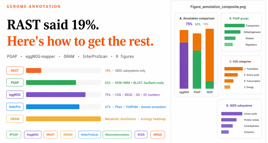
This script produces a four-panel figure: Panel A (annotation comparison across methods), Panel B (PGAP functional groups), Panel C (eggNOG COG categories), Panel D (top SEED subsystems). It also writes all data to a supplementary Excel file.
Libraries
library(tidyverse)
library(cowplot)
library(writexl)
library(scales)
library(forcats)
library(stringr)
Read input files
eggnog_file <- "Radiobacillus_eggnog.emapper.annotations"
pgap_file   <- "pgap_annotations.tsv"

# Read PGAP annotation table
pgap <- read_tsv(
  pgap_file,
  col_names = c("Gene_ID", "Product"),
  show_col_types = FALSE
) %>%
  mutate(
    Product     = replace_na(Product, "NA"),
    hypothetical = str_to_lower(Product) == "hypothetical protein"
  )

# Read eggNOG — skip comment lines, use the #query header
egg_lines   <- readLines(eggnog_file)
header_line <- egg_lines[str_detect(egg_lines, "^#query")][1]
header_vec  <- str_split(str_remove(header_line, "^#"), "\t")[[1]]

eggnog <- read_tsv(
  eggnog_file,
  comment = "#",
  col_names = header_vec,
  show_col_types = FALSE
)
Calculate summary statistics
pgap_total <- nrow(pgap)
pgap_hyp   <- sum(pgap$hypothetical, na.rm = TRUE)
pgap_annot <- pgap_total - pgap_hyp
pgap_pct   <- 100 * pgap_annot / pgap_total

eggnog_total <- nrow(eggnog)
eggnog_annot <- eggnog %>%
  mutate(Description = replace_na(Description, "-")) %>%
  summarise(n = sum(Description != "-" & Description != "")) %>%
  pull(n)
eggnog_unannot <- eggnog_total - eggnog_annot
eggnog_pct     <- 100 * eggnog_annot / eggnog_total

# SEED values from RAST output (fill these in from your RAST report)
seed_total   <- 5077
seed_annot   <- round(seed_total * 0.19)
seed_unannot <- seed_total - seed_annot
seed_pct     <- 100 * seed_annot / seed_total

# Summary table
summary_tbl <- tibble(
  Method               = c("eggNOG-mapper", "PGAP", "SEED subsystem"),
  Total_features       = c(eggnog_total, pgap_total, seed_total),
  Annotated_features   = c(eggnog_annot, pgap_annot, seed_annot),
  Unannotated_features = c(eggnog_unannot, pgap_hyp, seed_unannot),
  Percent_annotated    = c(eggnog_pct, pgap_pct, seed_pct)
)
PGAP functional groups
pgap_groups <- tibble(
  Category = c(
    "Transporters", "Dehydrogenases", "Kinases",
    "Ribosomal proteins", "Regulators", "Hypothetical proteins"
  ),
  Pattern = c(
    "transporter|permease|ABC transporter|MFS transporter",
    "dehydrogenase",
    "kinase",
    "ribosomal",
    "transcription factor|response regulator|helix-turn-helix",
    "^hypothetical protein$"
  )
) %>%
  rowwise() %>%
  mutate(Count = sum(str_detect(pgap$Product,
                                regex(Pattern, ignore_case = TRUE)), na.rm = TRUE)) %>%
  ungroup() %>%
  arrange(desc(Count))
COG categories from eggNOG
cog_map <- c(
  C = "Energy production and conversion",
  E = "Amino acid transport and metabolism",
  G = "Carbohydrate transport and metabolism",
  J = "Translation, ribosomal structure",
  K = "Transcription",
  L = "Replication, recombination and repair",
  M = "Cell wall/membrane biogenesis",
  O = "Protein modification and turnover",
  P = "Inorganic ion transport and metabolism",
  R = "General function prediction only",
  S = "Function unknown",
  T = "Signal transduction",
  V = "Defense mechanisms"
)

cog_long <- eggnog %>%
  select(query, COG_category) %>%
  mutate(COG_category = replace_na(COG_category, "-")) %>%
  filter(COG_category != "-", COG_category != "") %>%
  mutate(COG_category = str_split(COG_category, "")) %>%
  unnest(COG_category) %>%
  filter(str_detect(COG_category, "[A-Z]")) %>%
  mutate(COG_description = recode(COG_category, !!!cog_map, .default = "Other"))

cog_summary <- cog_long %>%
  count(COG_category, COG_description, sort = TRUE, name = "Count")
SEED subsystem summary (from RAST report)
seed_summary <- tribble(
  ~SEED_category,                                          ~Count,
  "Amino Acids and Derivatives",                           253,
  "Protein Metabolism",                                    180,
  "Carbohydrates",                                         166,
  "Cofactors, Vitamins, Prosthetic Groups, Pigments",      115,
  "Nucleosides and Nucleotides",                           101,
  "DNA Metabolism",                                         57,
  "RNA Metabolism",                                         49,
  "Respiration",                                            45,
  "Fatty Acids, Lipids, and Isoprenoids",                   45,
  "Membrane Transport",                                     41,
  "Virulence, Disease and Defense",                         41,
  "Cell Wall and Capsule",                                  38,
  "Stress Response",                                        32,
  "Dormancy and Sporulation",                               31
) %>%
  arrange(desc(Count))
Shared plot theme
theme_pub <- theme_bw(base_size = 12) +
  theme(
    panel.grid   = element_blank(),
    axis.text    = element_text(color = "black"),
    axis.title   = element_text(face = "bold"),
    legend.title = element_text(face = "bold"),
    plot.margin  = margin(10, 5, 5, 5)
  )
Panel A: annotation comparison (stacked bar)
comp_long <- summary_tbl %>%
  select(Method, Annotated_features, Unannotated_features) %>%
  pivot_longer(cols = c(Annotated_features, Unannotated_features),
               names_to = "Status", values_to = "Count") %>%
  mutate(
    Status = recode(Status,
                    Annotated_features   = "Annotated",
                    Unannotated_features = "Unannotated / not assigned"),
    Method = factor(Method, levels = c("eggNOG-mapper", "PGAP", "SEED subsystem"))
  )

figA <- comp_long %>%
  group_by(Method) %>%
  mutate(percent = Count / sum(Count) * 100) %>%
  ungroup() %>%
  mutate(Status = factor(Status,
                         levels = c("Annotated", "Unannotated / not assigned"))) %>%
  ggplot(aes(x = Method, y = Count, fill = Status)) +
  geom_col(width = 0.72) +
  geom_text(aes(label = paste0(round(percent, 1), "%")),
            position = position_stack(vjust = 0.5),
            color = "white", size = 4) +
  scale_fill_manual(values = c("Annotated"                    = "#1b9e77",
                                "Unannotated / not assigned"   = "#d95f02")) +
  labs(x = NULL, y = "Number of genes / proteins", fill = NULL) +
  theme_pub +
  theme(axis.text.x = element_text(angle = 20, hjust = 1),
        legend.position = "top")
Panel B: PGAP functional groups
figB <- pgap_groups %>%
  mutate(Category = str_wrap(Category, width = 22),
         Category = fct_reorder(Category, Count)) %>%
  ggplot(aes(x = Count, y = Category)) +
  geom_col(width = 0.72, fill = "#1b9e77") +
  labs(x = "Gene count", y = NULL) +
  theme_pub +
  theme(axis.text.y = element_text(size = 9))
Panel C: COG categories (eggNOG top 8)
figC <- cog_summary %>%
  slice_head(n = 8) %>%
  mutate(Label = paste(COG_category, COG_description, sep = " — "),
         Label = str_wrap(Label, width = 34),
         Label = fct_reorder(Label, Count)) %>%
  ggplot(aes(x = Count, y = Label)) +
  geom_col(width = 0.72, fill = "#d95f02") +
  labs(x = "Protein count", y = NULL) +
  theme_pub +
  theme(axis.text.y = element_text(size = 8.5))
Panel D: SEED subsystems (top 8)
figD <- seed_summary %>%
  slice_head(n = 8) %>%
  mutate(SEED_category = str_wrap(SEED_category, width = 30),
         SEED_category = fct_reorder(SEED_category, Count)) %>%
  ggplot(aes(x = Count, y = SEED_category)) +
  geom_col(width = 0.72, fill = "#7570b3") +
  labs(x = "Feature count", y = NULL) +
  theme_pub +
  theme(axis.text.y = element_text(size = 8.5))
Assemble and save
panelA <- ggdraw(figA) +
  draw_label("A", x=0.01, y=0.99, hjust=0, vjust=1, fontface="bold", size=16)
panelB <- ggdraw(figB) +
  draw_label("B", x=0.01, y=0.99, hjust=0, vjust=1, fontface="bold", size=16)
panelC <- ggdraw(figC) +
  draw_label("C", x=0.01, y=0.99, hjust=0, vjust=1, fontface="bold", size=16)
panelD <- ggdraw(figD) +
  draw_label("D", x=0.01, y=0.99, hjust=0, vjust=1, fontface="bold", size=16)

right_stack <- plot_grid(panelB, panelC, panelD,
                         ncol = 1, align = "v", rel_heights = c(1, 1, 1))

combined_fig <- plot_grid(panelA, right_stack,
                          ncol = 2, rel_widths = c(1.15, 1.35), align = "h")

ggsave("Figure_annotation_composite.png", combined_fig,
       width = 12, height = 10, dpi = 600)
ggsave("Figure_annotation_composite.pdf", combined_fig,
       width = 12, height = 10)
Supplementary tables
supp_list <- list(
  "S1_method_summary"   = summary_tbl,
  "S1_pgap_annotations" = pgap,
  "S1_pgap_groups"      = pgap_groups,
  "S1_eggnog_full"      = eggnog,
  "S1_COG_summary"      = cog_summary,
  "S1_SEED_summary"     = seed_summary
)

write_xlsx(supp_list, "Supplementary_Table_S1_Radiobacillus.xlsx")
Quick comparison: all five tools side by side
| Tool | Approach | Input | Main output | Best for |
|---|---|---|---|---|
| RAST | Curated subsystems | FASTA | Subsystem categories | Quick first look, ecological table |
| PGAP | NCBI HMM + BLAST | FASTA | GenBank, GFF3, FAA | Primary manuscript annotation |
| eggNOG-mapper | Ortholog groups (DIAMOND) | Protein FAA | COG, KEGG, GO, EC | Functional depth, COG plots |
| DRAM | Multi-DB metabolic distillation | FASTA | Metabolism heat map | Ecological interpretation |
| InterProScan | 13 domain databases | Protein FAA | Pfam, TIGRFAM, GO | Domain annotation, hypothetical proteins |
What to put in your manuscript
Table 1 (genome statistics): Include a row for each tool — total features, annotated, percentage.
Main figure: The four-panel figure produced by the R script above — annotation comparison (A), functional groups (B), COG categories (C), SEED subsystems (D).
Supplementary: The full eggNOG annotation table, the full PGAP product list, and the COG/SEED summaries.
Methods section:
Genome annotation was performed using NCBI PGAP (version X.X) run via Docker. Functional annotation was extended using eggNOG-mapper v2 (version X.X) with DIAMOND search against the eggNOG 5.0 database. Metabolic potential was assessed using DRAM (version X.X). Protein domain assignments were obtained using InterProScan (version X.X) against Pfam, TIGRFAM, and SUPERFAMILY databases. Subsystem-based interpretation was performed using the RAST/SEED annotation service.
A note on “hypothetical proteins”
One more thing beginners often worry about: you might have 35% hypothetical proteins after PGAP, 25% after eggNOG, and you wonder if that makes the genome look bad.
It does not. In most environmental bacterial genomes published today, 20–40% hypothetical proteins is completely normal. These are genes that are real (they pass gene-calling filters, they have Shine-Dalgarno sequences, they are conserved across strains) but simply have no characterised homolog yet. As more environmental bacteria are sequenced and characterised, these numbers will improve.
In your manuscript, frame it positively: “Our analysis revealed X% hypothetical proteins, consistent with the novel ecological niche of this organism and suggesting a reservoir of uncharacterised functional diversity.”
This workflow was developed during annotation of Radiobacillus sp. PE-A8-2. The same pipeline applies to any novel prokaryotic genome — adapt species names and file names accordingly. PGAP requires ~60–80 GB disk space; eggNOG databases require ~50 GB.
Tags: PGAP eggNOG-mapper RAST DRAM InterProScan genome-annotation COG KEGG ggplot2 hypothetical-proteins bioinformatics beginner