From Counts to Biology: A Rigorous DESeq2 Workflow for Multi-Factor Environmental Metatranscriptomics
🧬 𝐷𝑎𝑦 84 𝑜𝑓 𝐷𝑎𝑖𝑙𝑦 𝐵𝑖𝑜𝑖𝑛𝑓𝑜𝑟𝑚𝑎𝑡𝑖𝑐𝑠 𝑓𝑟𝑜𝑚 𝐽𝑜𝑗𝑦’𝑠 desk
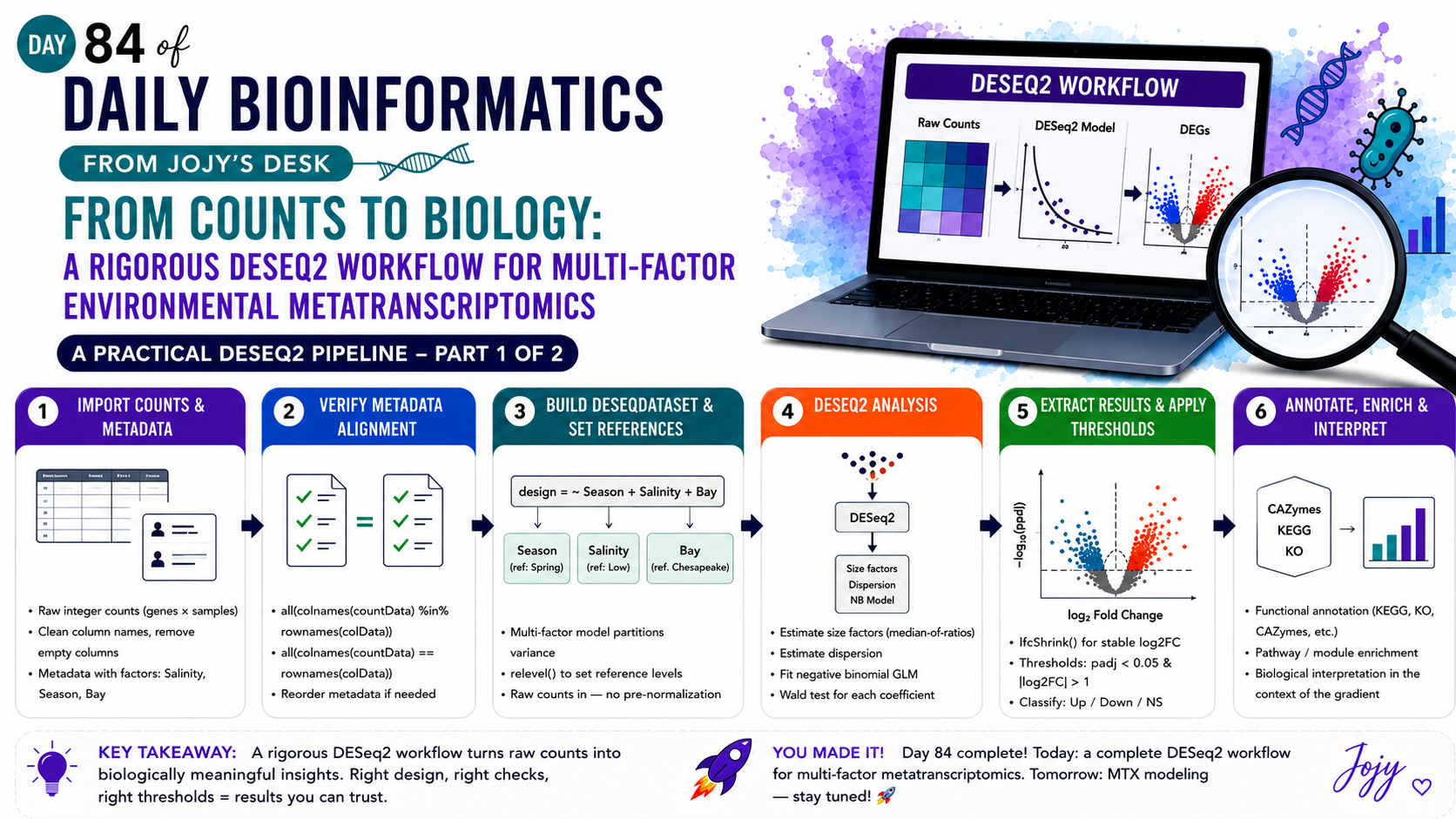
A virus detected in a metagenome might be dormant. A transcript detected in a metatranscriptome is evidence of something happening right now. The same logic applies to any functional gene: presence in DNA tells you what a community could do; expression in RNA tells you what it is doing. Differential expression analysis is how we move from that RNA signal to a ranked, statistically credible list of genes that respond to an environmental gradient. This post documents a complete DESeq2 workflow across three factors — salinity, season, and bay of origin — and covers every decision that determines whether the results are trustworthy.
Why DESeq2, and not TPM or fold-change on raw counts?
A common shortcut is to normalize counts to TPM or FPKM and then compare ratios between conditions. This fails for a fundamental reason: RNA-seq data is compositional. Library sizes differ between samples, the sequencing depth varies, and a small number of highly expressed genes can dominate the count distribution. Ad hoc normalization does not account for this in a statistically principled way.
DESeq2 uses median-of-ratios normalization, which estimates a size factor for each sample from the geometric mean of all genes. This is robust to outlier genes and compositional effects. Crucially, the normalization happens inside DESeq() — you should never pre-normalize your counts before passing them to DESeq2. The model assumes raw integer counts, and feeding it floats from a pre-normalized matrix breaks the negative binomial variance structure silently.
Raw counts in. Normalized, size-factor-corrected, dispersion-modeled results out. Do not shortcut the middle.
Step 1 — Import counts and metadata
library(DESeq2)
library(dplyr)
library(tibble)

### Import count table (raw integer counts, genes as rows, samples as columns)
countData <- read.table(
  "~/Desktop/Functional_redundancy/MT_deseq/attachments/raw_count_metabolism_updated.csv",
  header = TRUE, row.names = 1, sep = ","
)

### Import metadata
colData <- read.table(
  "~/Desktop/Functional_redundancy/MT_deseq/attachments/metadata.csv",
  header = TRUE, sep = ","
)
Two things to confirm before proceeding:
-
countDatashould contain only numeric columns — no gene annotation columns, no empty trailing columns (X,X.1) imported from Excel. Drop them withdf <- df[, !(names(df) %in% c("X", "X.1"))]. - Row names of
colDatamust correspond to column names ofcountData. If you setrow.names = 1when reading metadata, verify this was applied correctly.
Step 2 — Verify metadata alignment (non-negotiable)
Sample order mismatch between the count matrix and the metadata is one of the most damaging and hardest-to-detect errors in DGE analysis. If “S1” in column 3 of your count table maps to a different row in colData, every comparison is scrambled — and DESeq2 will not warn you.
# Both must return TRUE before building the DESeqDataSet
all(colnames(countData) %in% rownames(colData))  # all samples present?
all(colnames(countData) == rownames(colData))     # same order?
If the second check fails, reorder:
colData <- colData[colnames(countData), ]
all(colnames(countData) == rownames(colData))  # now TRUE
This is not defensive programming — it is the minimum required to trust your results.
Step 3 — Build DESeqDataSet objects and set reference levels
Three separate analyses are run, one per environmental factor. Each gets its own DESeqDataSet with the appropriate design formula and an explicit reference level set via relevel().
### Salinity: reference = Low
dds <- DESeqDataSetFromMatrix(
  countData = countData,
  colData   = colData,
  design    = ~ Salinity
)
dds$Salinity <- relevel(dds$Salinity, ref = "Low")

### Season: reference = Spring
ddsea <- DESeqDataSetFromMatrix(
  countData = countData,
  colData   = colData,
  design    = ~ Season
)
ddsea$Season <- relevel(ddsea$Season, ref = "Spring")

### Bay: reference = Chesapeake
ddbay <- DESeqDataSetFromMatrix(
  countData = countData,
  colData   = colData,
  design    = ~ Bay
)
ddbay$Bay <- relevel(ddbay$Bay, ref = "Chesapeake")
Why relevel() matters: Without it, DESeq2 defaults to alphabetical factor ordering. “High” comes before “Low” alphabetically, so fold-changes would be reported as High/Low rather than the biologically intuitive Low-as-baseline direction. Getting this wrong does not produce an error — it inverts your fold-changes and your biological interpretation.
When to use a multi-factor design: If salinity and season are confounded in your sampling design (e.g., high-salinity samples were consistently collected in summer), a single-factor model will conflate their effects. The appropriate design in that case would be design = ~ Season + Salinity, which partitions variance from each factor separately. Inspect your metadata and a PCA before deciding.
Step 4 — Run DESeq2
The core analysis is a single call. DESeq2 sequentially estimates size factors, fits dispersion, and runs the negative binomial GLM.
dds   <- DESeq(dds)
ddsea <- DESeq(ddsea)
ddbay <- DESeq(ddbay)
Always call resultsNames() before extracting results. This verifies that DESeq2 encoded your factor levels as intended.
resultsNames(dds)
# [1] "Intercept"            "Salinity_High_vs_Low" "Salinity_Medium_vs_Low"
A mislabeled contrast — or one you never noticed was inverted — means every fold-change interpretation is backwards.
Step 5 — Extract results with named contrasts
# Default results object (last factor level vs. reference)
res <- results(dds)

# Explicit pairwise contrasts
res_high_vs_low <- results(dds, name = "Salinity_High_vs_Low")
res_med_vs_low  <- results(dds, name = "Salinity_Medium_vs_Low")
For downstream plotting and export, convert to data frames and add gene IDs as an explicit column:
res_df       <- as.data.frame(res)
res_df$gene  <- rownames(res_df)
Step 6 — Statistical thresholds
Two thresholds define a differentially expressed gene. Both must be applied together.
| Threshold | Value | Rationale |
|---|---|---|
| Adjusted p-value (FDR) | padj < 0.05 | Controls false discovery rate across genome-scale testing. Raw p-values are not appropriate — with 10,000 features tested, p < 0.05 yields ~500 false positives by chance. |
| Absolute log₂ fold-change | abs(log2FoldChange) > 1 | Filters statistically significant but biologically trivial changes. A twofold threshold is standard; 0.58 (~1.5-fold) is used in some contexts. |
# Summarize at FDR = 0.05
summary(results(dds, alpha = 0.05))

# Filter significant DEGs
sig_genes <- res_df |>
  filter(!is.na(padj), padj < 0.05, abs(log2FoldChange) > 1)
A gene that passes only one threshold is not a confident hit. High statistical significance at a trivially small fold-change is a feature of high-depth studies, not a biological signal.
Step 7 — Combining results across factors for comparison
To compare the transcriptional response across all three factors simultaneously, results are combined into a long-format data frame tagged by factor:
res_sal <- results(dds)   |> as.data.frame() |> mutate(Factor = "Salinity", Gene = rownames(results(dds)))
res_sea <- results(ddsea) |> as.data.frame() |> mutate(Factor = "Season",   Gene = rownames(results(ddsea)))
res_bay <- results(ddbay) |> as.data.frame() |> mutate(Factor = "Bay",      Gene = rownames(results(ddbay)))

res_all_clean <- bind_rows(res_sal, res_sea, res_bay) |>
  filter(!is.na(padj)) |>
  mutate(
    ShortName = stringr::str_extract(Gene, "(?<=\\().+?(?=\\))"),
    ShortName = ifelse(is.na(ShortName), Gene, ShortName)
  )
The ShortName extraction pulls abbreviated names from parentheses in gene identifiers (e.g., "nitrite reductase (nirS)" → "nirS"), falling back to the full gene name when no abbreviation is present. This keeps volcano plot labels readable.
Step 8 — Integrating functional annotation
Raw gene identifiers without context have limited interpretive value. DESeq2 results are joined to a functional annotation table that classifies genes into categories — metabolic markers and CAZymes (carbohydrate-active enzymes) in this study:
annotation <- read.csv(
  "~/Desktop/Functional_redundancy/MT_deseq/attachments/Annotations.csv",
  header = TRUE
)

# Merge DESeq2 results with annotation
res_annot  <- merge(res_df, annotation, by = "gene")

# Subset by functional category
metabolic_res <- subset(res_annot, category == "mmarker")
cazy_res      <- subset(res_annot, category == "CAZY")

write.csv(metabolic_res, "DESeq2_metabolic_markers.csv", row.names = FALSE)
write.csv(cazy_res,      "DESeq2_CAZy.csv",              row.names = FALSE)
This keeps every result traceable: each reported gene links back to its annotation, its fold-change, and its adjusted p-value.
Step 9 — Visualization: faceted volcano plots
A volcano plot serves two purposes: it communicates the scale and direction of differential expression, and it functions as a quality-control check. Before interpreting biology, inspect the plot for these red flags:
- One-sided volcano (all hits in one direction): suggests a normalization problem or a metadata label swap.
- Asymmetric point cloud: can indicate batch effects or compositional biases that the single-factor model hasn’t captured.
- Top-labeled genes that don’t make biological sense: warrants investigation before publication.
library(ggplot2)
library(ggrepel)

sig_genes_plot <- res_all_clean |> filter(padj < 0.05)

ggplot(res_all_clean, aes(x = log2FoldChange, y = -log10(padj))) +
  geom_point(aes(color = padj < 0.05), alpha = 0.6) +
  geom_text_repel(
    data         = sig_genes_plot,
    aes(label    = ShortName),
    size         = 3,
    max.overlaps = Inf,
    box.padding  = 0.3,
    point.padding = 0.2,
    segment.color = "grey50"
  ) +
  facet_wrap(~ Factor, scales = "free_x") +
  scale_color_manual(values = c("grey", "red")) +
  labs(
    title  = "Differential Abundance by Factor",
    x      = "Log2 Fold Change",
    y      = "-Log10 Adjusted P-value",
    color  = "Significant (padj < 0.05)"
  ) +
  theme_bw() +
  theme(
    panel.grid.major = element_blank(),
    panel.grid.minor = element_blank(),
    legend.position  = "bottom"
  )
Faceting by factor in a single figure lets reviewers immediately see which environmental variable carries the largest transcriptional signal in this dataset.
The ten-point reproducibility checklist
Before sharing or submitting results, verify each of the following. These are not suggestions — they are the checks that catch the errors that invalidate analyses.
-
all(colnames(countData) == rownames(colData))returnsTRUE. - Reference levels are explicitly set with
relevel()for all factor variables. - Contrast names are verified with
resultsNames()before anyresults()call. - Raw integer counts are used as input — not TPM, FPKM, or pre-normalized values.
- Adjusted p-values (FDR/BH) are used for filtering, not raw p-values.
- Both
padjandlog2FoldChangethresholds are applied when defining significant DEGs. - PCA, dispersion plot, and MA plot have been visually inspected for outliers and batch effects.
- Low-count genes have been filtered (e.g.,
rowSums(counts >= 10) >= Nappropriate for your sample size) before running DESeq2. - All output files, scripts, and input data are saved with consistent, descriptive filenames.
-
sessionInfo()output is saved alongside all result files.
# Always run this at the end of your analysis script
sessionInfo()
Biological interpretation: what the numbers actually say
Statistical significance and biological significance are not the same thing. A gene with padj = 1×10⁻²⁰ and log2FC = 0.3 is a trivially small change with enormous statistical power behind it. A gene with padj = 0.04 and log2FC = 3.2 is a large change that barely cleared the FDR threshold. Both thresholds exist because we need both: statistical rigor to control false discovery rates, and effect-size filtering to focus on changes worth interpreting.
In environmental metatranscriptomics, the “genes” being tested are often metabolic pathway markers or functional gene families rather than single-organism transcripts. A significant increase in CAZyme-encoding transcripts under high salinity does not mean a single organism is responding — it means the community-level functional capacity shifted. Interpretation must be grounded in the ecological question.
Treat DESeq2 output as a ranked list of candidates that are worth investigating, not a list of confirmed biological findings. Cross-check significant gene names against curated databases (KEGG, CAZy, DRAM-v), confirm pathway membership manually, and evaluate whether the biology is consistent with what is known about your system.
Summary
| Step | What it does | Why it matters |
|---|---|---|
| Metadata alignment check | Verifies sample order | Mismatch invalidates all results |
relevel() | Sets biologically meaningful reference | Prevents inverted fold-changes |
resultsNames() | Verifies contrast encoding | Catches mislabeled comparisons |
| Raw counts as input | Enables DESeq2 normalization | Pre-normalized values break the model |
| FDR threshold | Controls false discovery rate | Raw p-values are invalid at genomic scale |
| log2FC threshold | Filters trivially small changes | Large N studies produce many tiny-effect hits |
| Functional annotation merge | Connects statistics to biology | Gene IDs alone are uninterpretable |
sessionInfo() | Records package versions | Required for reproducibility |
The value of a careful DESeq2 workflow is not that it answers biological questions. It is that it produces a credible, traceable, reproducible list of candidates that are worth the effort of answering.
Analysis performed using DESeq2 (Love, Huber & Anders 2014, Genome Biology 15:550). All code verified against current Bioconductor documentation. Raw data, annotated scripts, and sessionInfo() output should accompany any publication of these results.