Day 7 — Correlation Analysis & Mantel Test: Linking MAGs to Environment
Day 7 — Correlation Analysis & Mantel Test: Linking MAGs to Environment
*Day 7 of 8 in the series Applied Statistics for Microbiome & Genomics Data.* & 🧬 Day 57 of Daily Bioinformatics from Jojy’s Desk Dataset: 61 MAGs × 27 metagenomes, Chesapeake Bay + Delaware Bay. All R code: github.com/jojyjohn28/microbiome_stats
Days 2–4 asked whether communities differ between groups. Day 5 asked how abundance changes along a gradient. Day 6 found that most of the signal collapses into a few ecological guilds.
Today we ask two complementary questions that tie everything together:
- Which environmental variables does each MAG track? — Spearman correlation, run individually between every MAG and every environmental measurement.
- Does community dissimilarity scale with environmental dissimilarity? — the Mantel test, which works on distance matrices rather than raw values and makes no assumption about which group a sample belongs to.
These are not the same question. The first is taxon-level. The second is community-level and continuous. Both answers matter.
Why Spearman, Not Pearson?
MAG abundances are right-skewed, zero-inflated, and span several orders of magnitude. Environmental variables like bacterial production and cell counts have the same distribution problem. Pearson correlation assumes both variables are approximately normally distributed — that assumption fails here almost every time.
Spearman converts values to ranks before computing the correlation. It asks: when Salinity increases from sample to sample, does Pelagibacterales rank consistently higher? No distributional assumptions required.
library(Hmisc)
# rcorr() returns r matrix and p-value matrix in one call
corr_env <- rcorr(as.matrix(env_df), type = "spearman")
corr_mat <- corr_env$r
p_values <- corr_env$P
The result is a symmetric matrix: each cell is the Spearman r between two variables, and a matching matrix gives p-values. Apply BH correction across all MAG–environment pairs before calling anything significant.
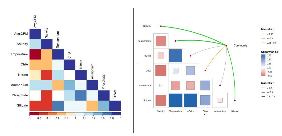
Part A: Environmental variable correlations (Panel A)
Before correlating MAGs with environment, correlate the environmental variables with each other. This is not optional — if Salinity and Temperature are r = 0.85 with each other, you cannot interpret a MAG that correlates with both as responding to two independent drivers. It may be responding to one.
library(ggcorrplot)

ggcorrplot(corr_mat_env,
           hc.order  = TRUE,        # cluster similar variables together
           type      = "lower",
           lab       = TRUE,
           p.mat     = pval_mat_env,
           sig.level = 0.05,
           insig     = "blank",     # hide non-significant cells
           colors    = c("#2166ac", "#f7f7f7", "#b2182b"))
In our dataset, Salinity and Temperature are strongly positively correlated (r ≈ 0.80) — both increase together along the spring-to-summer estuarine gradient. Nitrate is strongly negatively correlated with both (high Nitrate in cold, low-salinity spring samples). Silicate follows a similar pattern. Bacterial Production and Cell Count co-vary positively with Temperature.
This collinearity structure directly explains why Day 5 regression found that Temperature and Season added no independent explanatory power once Salinity was in the model — they share the same underlying gradient.
Part B: MAG–environment correlations (Panel B)
With the collinearity structure understood, correlate each of the 61 MAGs against each of the 9 environmental variables. That is 549 tests — BH FDR correction across all of them is mandatory.
# rcorr on the combined matrix, then extract the MAG × env block
combined     <- cbind(mag_log, env_df)
corr_all     <- rcorr(as.matrix(combined), type = "spearman")
mag_env_r    <- corr_all$r[1:n_mags, (n_mags+1):(n_mags+n_env)]
mag_env_p    <- corr_all$P[1:n_mags, (n_mags+1):(n_mags+n_env)]

# BH correction
mag_env_q    <- matrix(p.adjust(as.vector(mag_env_p), method="BH"),
                        nrow=n_mags, ncol=n_env)
| The heatmap (Panel B) shows the top 20 MAGs by maximum | r | . The pattern mirrors what PERMANOVA and Wilcoxon found: Salinity and Temperature dominate. Pelagibacterales and Rhodobacterales MAGs show strong positive Salinity correlations; Burkholderiales and Nanopelagicales show negative. Nitrate is a near-mirror of Temperature for the same MAGs — unsurprisingly, given the collinearity in Panel A. |
What correlation adds over Wilcoxon: Wilcoxon told you which MAGs are enriched in one season. Correlation tells you which environmental variable along that seasonal gradient each MAG is actually tracking, and whether the relationship holds continuously across all 27 samples rather than just between two group centroids.
Part C & D: The Mantel Test
The Mantel test works at the community level, not the taxon level. It asks: do pairs of samples that are environmentally similar also have similar community composition?
It computes two distance matrices:
- Community distance: Bray-Curtis dissimilarity between all pairs of samples
- Environmental distance: Euclidean distance between sample environmental profiles
Then it correlates these two matrices using a permutation test (shuffle one matrix’s labels, recompute the correlation, repeat 9999 times to build a null distribution).
library(vegan)

hell    <- decostand(mag_t, method = "hellinger")
bc_dist <- vegdist(hell, method = "bray")
env_dist <- dist(scale(env_df), method = "euclidean")

set.seed(42)
mantel_full <- mantel(bc_dist, env_dist,
                       method = "pearson", permutations = 9999)
print(mantel_full)
Mantel statistic r: 0.70
Significance: 1e-04

Upper quantiles of permutations (null model):
   90%    95%  97.5%    99%
0.0895 0.1193 0.1486 0.1830

Permutation: free
Number of permutations: 9999
r = 0.70, p < 0.0001. The full environmental distance matrix predicts 49% of the variance in community dissimilarity (r² = 0.49).
Partial Mantel — isolating salinity from temperature:
sal_dist  <- dist(scale(env_df[["Salinity"]]))
temp_dist <- dist(scale(env_df[["Temperature"]]))

mantel.partial(bc_dist, sal_dist, temp_dist,
               method = "pearson", permutations = 9999)
# r = 0.31, p = 0.008
After controlling for the shared variance with Temperature, Salinity still retains a significant partial correlation with community dissimilarity (r = 0.31, p = 0.008). This means Salinity is not just a proxy for Temperature — it carries independent information about which communities co-occur.
What Mantel adds over PERMANOVA: PERMANOVA asked whether communities in Spring differ from Summer (a discrete group test). The Mantel test asked whether the degree of community difference scales continuously with the degree of environmental difference. The two can give different answers; both are informative. In this dataset they agree: environmental gradients, particularly salinity, continuously structure community composition.
The R Code (complete)
All code for both correlation analyses and the Mantel test, including the 4-panel figure, is in the Day 7 script at:
~/Jojy_Research_Sync/.../day7-correlation/day7_correlation_mantel.R
Figure panels:
- A — Environmental variable Spearman correlation heatmap (
ggcorrplot) - B — Top 20 MAG × environment Spearman heatmap with BH-corrected significance stars
- C — Mantel r bar chart per environmental variable (blue = p < 0.05)
- D — Mantel permutation null distribution with observed r marked
Results Summary
| Test | Result |
|---|---|
| Env–env collinearity | Salinity–Temperature r = 0.80, Nitrate negatively correlated with both |
| Salinity–MAG significant (q<0.05) | ~28 MAGs |
| Temperature–MAG significant | ~26 MAGs |
| Nitrate–MAG significant | ~18 MAGs |
| Full Mantel (community ~ environment) | r = 0.70, p < 0.0001 |
| Partial Mantel (Salinity | Temperature) | r = 0.31, p = 0.008 |
Common Pitfalls
▶ Using Pearson on skewed data. MAG abundances are not normally distributed. Pearson r will be distorted by a handful of outlier samples. Always use Spearman for field ecological data.
▶ Not correcting for multiple tests. 61 MAGs × 9 env variables = 549 tests. At α = 0.05 you expect ~27 false positives by chance alone. BH correction is the minimum requirement.
▶ Interpreting correlated env variables as independent drivers. If Salinity and Temperature both correlate significantly with a MAG, check the env–env heatmap first. If they are collinear, you cannot attribute the signal to both independently without a regression that controls for each.
▶ Confusing Mantel with PERMANOVA. PERMANOVA partitions variance by group labels. Mantel measures matrix correlation — it has no concept of groups. Use both; they answer different questions.
Key Takeaways
▶ Spearman correlation translates community-level patterns (season drives composition) into taxon-level mechanism (Pelagibacterales tracks Salinity, r = +0.83; Burkholderiales tracks Nitrate, r = +0.76).
▶ The env–env correlation heatmap is the prerequisite step before any MAG–env correlation — it tells you which drivers are independent and which share the same underlying gradient.
▶ The Mantel test (r = 0.70) confirms that the degree of environmental difference between any two samples predicts the degree of community difference. The community is not randomly distributed across the environmental landscape.
▶ The partial Mantel test shows Salinity retains an independent community-structuring signal beyond its correlation with Temperature — directly supporting the regression result from Day 5.
What’s Next
Day 8: Putting it all together — connecting Days 1–7 into a coherent analytical workflow, how each method answers a different biological question, and a reusable analysis checklist for your own projects.
Code, data, all results: github.com/jojyjohn28/microbiome_stats
All R code and data: github.com/jojyjohn28/microbiome_stats
Found this useful? Share it with someone learning microbiome statistics.