Day 5 — Multiple Regression for MAG Abundance: Linking Genomics to Environment
Day 5 — Multiple Regression for MAG Abundance: Linking Genomics to Environment
*Day 5 of 7 in the series Applied Statistics for Microbiome & Genomics Data.* & 🧬 Day 55 of Daily Bioinformatics from Jojy’s Desk Dataset: 61 MAGs × 27 metagenomes, Chesapeake Bay + Delaware Bay. All R code: github.com/jojyjohn28/microbiome_stats
Days 2–4 were about categories. PERMANOVA told us communities differ by season. Wilcoxon told us 40 of 61 MAGs are significantly enriched in one season over another. Both approaches treat season as a discrete label — Spring or Summer, group A or group B.
Today we ask a fundamentally different question:
How does a MAG’s abundance change as salinity increases by 1 psu? Does that relationship hold at all seasons, or only in summer? How much of the variance can we actually explain?
This is multiple regression — the bridge from discrete group comparisons to the continuous environmental gradients that actually structure microbial communities in estuaries. It also forces us to be honest about model assumptions in a way that Wilcoxon tests do not.
Why Not Just Use Wilcoxon for Everything?
The Wilcoxon test compares ranks between two groups. It cannot tell you:
- How much abundance changes per unit of salinity or temperature
- Whether salinity is a better predictor than temperature, after accounting for both simultaneously
- Whether the salinity–abundance relationship is steeper in summer than spring (an interaction)
- Which fraction of total variance each environmental variable explains independently
Regression answers all of these. The trade-off is stronger assumptions — and an obligation to check them every time.
Four MAGs, Four Ecological Stories
We focus on four MAGs with clear a priori hypotheses:
▶ Pelagibacterales MAG 18 — SAR11 clade, the most abundant marine bacteria on Earth. Expected to increase strongly with salinity, since these are canonical marine specialists that thrive in high-salinity offshore waters.
▶ Nanopelagicales MAG 18 — acI lineage, freshwater actinobacteria. Expected to decrease with salinity — found in rivers and low-salinity estuarine zones, disappearing as marine water dominates.
▶ Flavobacteriales MAG 6 — particle-degrading bacteria linked to phytoplankton blooms. Expected to track season (bloom timing, organic matter availability) more than the salinity gradient itself.
▶ Rhodobacterales MAG 15 — Roseobacter clade, metabolically versatile. Expected to respond to salinity but potentially also to organic matter proxies like chlorophyll.
Before You Model Anything: Plot It
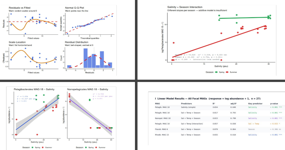
▶ The first thing you should always do is scatter-plot the response against each predictor, coloured by season. Panels A and B show these relationships for Pelagibacterales and Nanopelagicales against salinity.
▶ The contrast is striking. Pelagibacterales (Panel A) increases monotonically with salinity — r² = 0.654 on a single-variable regression, β = +0.327 per psu, p < 0.001. Nanopelagicales (Panel B) shows the exact mirror image — r² = 0.769, β = −0.325 per psu, p < 0.001. Same magnitude of effect, opposite sign, opposite ecological strategy.
▶ Notice that the points are coloured by season but the regression line ignores season entirely. Low-salinity samples are all Spring; high-salinity samples are all Summer. Salinity and season are correlated in this estuary. This will matter enormously when we add both to a single model.
The Statistical Framework
The additive linear model
The core equation for multiple regression with three predictors:
log(abundance + 1) = β₀ + β₁·Salinity + β₂·Temperature + β₃·Season + ε
- β₀ — intercept: predicted log-abundance when all predictors equal zero
- β₁ — salinity coefficient: expected change in log-abundance for a 1 psu increase in salinity, holding Temperature and Season constant
- β₂ — temperature coefficient: same logic for temperature
- β₃ — season coefficient: expected difference between Summer (coded 1) and Spring (coded 0) after controlling for Salinity and Temperature
- ε — residual error: everything not captured by the model
The word additive is critical. This model assumes the effect of salinity is identical at all temperatures and in both seasons. If that assumption is wrong — and in ecology it often is — you need an interaction term.
Why log-transform first?
Raw MAG abundance values are right-skewed, zero-inflated, and span four or more orders of magnitude. Fitting OLS on untransformed counts often violates linearity and residual assumptions, which can substantially distort coefficient estimates, standard errors, and p-values.. After log1p(x) transformation:
- The response variable is approximately normally distributed
- Relationships with continuous predictors become approximately linear
- Coefficients have a clean multiplicative biological interpretation
Interpreting β coefficients biologically
For Pelagibacterales MAG 18, the additive multiple regression (Salinity + Temperature + Season) gives β_Salinity = +0.271 (SE = 0.039, t = 6.98, p < 0.001).
This means: for every 1 psu increase in salinity, log(Pelagibacterales MAG 18 + 1) increases by 0.271 units, after accounting for Temperature and Season.
In original abundance units, exponentiate: e^0.271 ≈ 1.31 — a 31% increase in abundance per 1 psu of salinity. Across the full salinity range in our dataset (0.18 to 30.52 psu = 30.3 units): 0.271 × 30.3 ≈ 8.2 log units of predicted change. That is the difference between near-zero and the highest abundances in our dataset — entirely consistent with a marine specialist traversing an estuarine gradient from freshwater to marine conditions.
For Nanopelagicales MAG 18, βSalinity = −0.349 (t = −9.65, p < 0.001). Every 1 psu increase in salinity corresponds to a 29% _decrease in abundance. Two perfectly contrasting ecological strategies, captured by slope sign alone.
Partial vs simple coefficients
Notice that βSalinity in the additive model (0.271) is slightly smaller than in the simple regression (0.327). This is because the additive model _partials out the shared variance between Salinity, Temperature, and Season. The simple regression overestimates the salinity effect because it absorbs variance that is actually due to Temperature and Season (which happen to be collinear with Salinity in this estuary).
Neither estimate is “wrong” — they answer different questions. Simple regression answers: “how does abundance change with salinity in this dataset?” Multiple regression answers: “how does abundance change with salinity independent of Temperature and Season?” The latter is usually what you want biologically.
R² and adjusted R²
R² is the proportion of variance explained. The additive model explains R² = 0.817 of Pelagibacterales variance — strong for field ecological data. Adding Temperature and Season on top of Salinity alone increased R² from 0.654 to 0.817.
Always report adjusted R², which penalises for additional predictors. Here adj.R² = 0.793, not far below R² = 0.817, confirming Temperature and Season are genuinely contributing rather than just inflating the statistic.
The R Code
Setup: load, align, log-transform
library(vegan)
library(ggplot2)
library(patchwork)
library(broom)   # tidy model outputs
library(car)     # vif() multicollinearity check
library(lmtest)  # bptest() heteroscedasticity

# Load data
metadata <- read.csv("../day1/data/metadata.csv", header=TRUE, row.names=1, sep=",")
mag_raw  <- read.csv("../day1/data/mag_abundance.csv", header=TRUE, row.names=1, sep=",")
mag_t    <- t(mag_raw)

# Align — always verify before proceeding
metadata <- metadata[match(rownames(mag_t), rownames(metadata)), ]
stopifnot(all(rownames(mag_t) == rownames(metadata)))

# CRITICAL: log-transform before any regression
mag_log <- log1p(mag_t)

# Encode and derive predictors
metadata$Season_num  <- ifelse(metadata$Season == "Summer", 1, 0)
metadata$Sal_x_Temp  <- metadata$Salinity * metadata$Temperature

# Build modelling dataframe (n=27, no NAs for these variables)
reg_df <- cbind(
  metadata[, c("Season","Season_num","Salinity","Temperature","ChlA","Sal_x_Temp")],
  mag_log[, c("Pelagibacterales_MAG_18", "Nanopelagicales_MAG_18",
              "Flavobacteriales_MAG_6",  "Rhodobacterales_MAG_15")]
)
cat("n =", nrow(reg_df), "\n")  # 27
Always scatter-plot before modelling
scatter_pela <- ggplot(reg_df, aes(Salinity, Pelagibacterales_MAG_18, colour=Season)) +
  geom_point(size=3.5, alpha=0.9) +
  geom_smooth(method="lm", se=TRUE, colour="#1d4ed8", linewidth=1.4) +
  scale_colour_manual(values=c("Spring"="#16a34a","Summer"="#dc2626")) +
  annotate("text", x=1, y=11.5,
           label="r² = 0.654\nβ = +0.327 per psu\np < 0.001",
           hjust=0, size=3.5, family="mono", colour="#1d4ed8") +
  labs(x="Salinity (psu)", y="log(abundance + 1)",
       title="Pelagibacterales MAG 18 ~ Salinity") +
  theme_classic(base_size=12) + theme(legend.position="bottom")

scatter_nano <- ggplot(reg_df, aes(Salinity, Nanopelagicales_MAG_18, colour=Season)) +
  geom_point(size=3.5, alpha=0.9) +
  geom_smooth(method="lm", se=TRUE, colour="#7c3aed", linewidth=1.4) +
  scale_colour_manual(values=c("Spring"="#16a34a","Summer"="#dc2626")) +
  annotate("text", x=17, y=9.5,
           label="r² = 0.769\nβ = −0.325 per psu\np < 0.001",
           hjust=0, size=3.5, family="mono", colour="#7c3aed") +
  labs(x="Salinity (psu)", y="log(abundance + 1)",
       title="Nanopelagicales MAG 18 ~ Salinity") +
  theme_classic(base_size=12) + theme(legend.position="bottom")

scatter_pela | scatter_nano
Fit and inspect the additive models
# Model 1: Pelagibacterales ~ Salinity + Temperature + Season (additive)
m1 <- lm(Pelagibacterales_MAG_18 ~ Salinity + Temperature + Season_num,
          data=reg_df)
summary(m1)
Coefficients:
              Estimate Std. Error t value Pr(>|t|)
(Intercept)    5.9801     2.0368    2.94   0.0074 **
Salinity       0.2706     0.0387    6.98  < 0.001 ***
Temperature   -0.0753     0.2142   -0.35   0.728
Season_num    -2.7203     4.0252   -0.68   0.506

Residual standard error: 1.671 on 23 df
R² = 0.8171   Adjusted R² = 0.7933
Salinity is the only significant predictor (p < 0.001). Temperature and Season are not significant after accounting for Salinity — because all three variables travel together up the estuarine gradient. As summer arrives, freshwater input drops, salinity rises, and temperature rises. The same gradient, measured three ways. Once Salinity is in the model, Temperature and Season add no independent explanatory power.
tidy(m1)    # broom: clean coefficient table with CIs
glance(m1)  # broom: R², AIC, BIC, etc.

# Biological interpretation
cat(sprintf(
  "β_Salinity = %.4f\nPer 1 psu: ×%.2f (%.0f%% change)\nFull range (30.3 psu): %.1f log-units\n",
  coef(m1)["Salinity"],
  exp(coef(m1)["Salinity"]),
  (exp(coef(m1)["Salinity"]) - 1) * 100,
  coef(m1)["Salinity"] * 30.3
))
# β_Salinity = 0.2706
# Per 1 psu: ×1.31 (31% change)
# Full range (30.3 psu): 8.2 log-units
# Model 2: Nanopelagicales — opposite salinity direction
m2 <- lm(Nanopelagicales_MAG_18 ~ Salinity + Temperature + Season_num,
          data=reg_df)
summary(m2)
# Salinity: β = -0.3488  t = -9.65  p < 0.001 ***
# R² = 0.815   adj.R² = 0.790

# Model 3: Flavobacteriales — season-dominant, not salinity
m3 <- lm(Flavobacteriales_MAG_6 ~ Salinity + Temperature + Season_num,
          data=reg_df)
summary(m3)
# R² = 0.879  adj.R² = 0.864
# NO individual predictor is significant (Season: β=-3.27, p=0.306)
# High R² with no significant individual predictors — joint collinear effect

# Model 4: Rhodobacterales — moderate salinity response
m4 <- lm(Rhodobacterales_MAG_15 ~ Salinity + Temperature + Season_num,
          data=reg_df)
summary(m4)
# Salinity: β = +0.1979  t = 4.07  p < 0.001 ***
# R² = 0.655   adj.R² = 0.610
Check multicollinearity
vif(m1)
#   Salinity  Temperature  Season_num
#      3.12         3.98        4.07
# All < 5 — acceptable. High VIF (>5–10) would destabilise coefficients.
The four diagnostic plots
These are not optional. Run them for every model you report.
# All four at once in base R
par(mfrow=c(2,2)); plot(m1); par(mfrow=c(1,1))

# Or rebuild in ggplot2 for publication quality:

# D: Residuals vs Fitted
p_D <- ggplot(data.frame(fitted=fitted(m1), resid=resid(m1)),
              aes(fitted, resid)) +
  geom_point(colour="#1d4ed8", size=2.5, alpha=0.8) +
  geom_hline(yintercept=0, colour="#dc2626", linetype="dashed", linewidth=1.2) +
  geom_smooth(method="loess", se=FALSE, colour="#d97706", linewidth=1.5) +
  labs(x="Fitted values", y="Residuals",
       title="Residuals vs Fitted",
       subtitle="Want: random scatter around 0") +
  theme_classic()

# E: Normal Q-Q
resids_std <- rstandard(m1)
p_E <- ggplot(data.frame(resids_std), aes(sample=resids_std)) +
  stat_qq(colour="#1d4ed8", size=2.5, alpha=0.8) +
  stat_qq_line(colour="#dc2626", linetype="dashed", linewidth=1.2) +
  labs(x="Theoretical quantiles", y="Sample quantiles",
       title="Normal Q-Q Plot",
       subtitle="Want: points near the line") +
  theme_classic()

# F: Scale-Location
p_F <- ggplot(data.frame(fitted=fitted(m1),
                          sqrt_abs=sqrt(abs(resid(m1)))),
              aes(fitted, sqrt_abs)) +
  geom_point(colour="#1d4ed8", size=2.5, alpha=0.8) +
  geom_smooth(method="loess", se=FALSE, colour="#d97706", linewidth=1.5) +
  labs(x="Fitted values", y="√|Residuals|",
       title="Scale-Location",
       subtitle="Want: flat horizontal band") +
  theme_classic()

# G: Residual histogram with normal overlay
r_df <- data.frame(r=resid(m1))
p_G <- ggplot(r_df, aes(r)) +
  geom_histogram(bins=11, fill="#1d4ed8", colour="white", alpha=0.65) +
  stat_function(fun=function(x)
    dnorm(x, mean(r_df$r), sd(r_df$r)) * nrow(r_df) * diff(range(r_df$r))/11,
    colour="#dc2626", linetype="dashed", linewidth=1.8) +
  geom_vline(xintercept=0, linetype="dotted") +
  labs(x="Residuals", y="Count",
       title="Residual Distribution",
       subtitle="Want: bell-shaped, centred at 0") +
  theme_classic()

(p_D | p_E) / (p_F | p_G)
# Formal tests to accompany the visuals
shapiro.test(resid(m1))
# W = 0.931  p = 0.081  — cannot reject normality (borderline; fine for n=27)

bptest(m1)   # Breusch-Pagan
# BP = 3.18  p = 0.364  — no evidence of heteroscedasticity
The interaction model
# Model 5: Pelagibacterales ~ Salinity × Temperature
# Tests whether the salinity slope differs at different temperatures
m5 <- lm(Pelagibacterales_MAG_18 ~ Salinity * Temperature, data=reg_df)
summary(m5)
Coefficients:
                    Estimate Std. Error t value Pr(>|t|)
(Intercept)         15.1328     3.3615    4.50  0.0002 ***
Salinity            -0.0811     0.1368   -0.59  0.559
Temperature         -0.5524     0.1347   -4.10  0.0004 ***
Salinity:Temperature 0.0148     0.0056    2.63  0.015 *

R² = 0.857   Adjusted R² = 0.838
The interaction term β_(Sal×Temp) = +0.0148 (p = 0.015) is significant. The salinity slope is not constant — it is steeper at higher temperatures. In summer (high temperature), each additional psu of salinity corresponds to even greater Pelagibacterales abundance than the additive model would predict.
Visualising this as separate seasonal lines (Panel H) makes the interaction concrete:
# H: Separate regression lines by season
p_int <- ggplot(reg_df, aes(Salinity, Pelagibacterales_MAG_18, colour=Season)) +
  geom_point(size=3.5, alpha=0.9) +
  geom_smooth(method="lm", se=FALSE, linewidth=2.2) +
  scale_colour_manual(values=c("Spring"="#16a34a","Summer"="#dc2626")) +
  annotate("text", x=1, y=0.8,
           label="Spring  β = +0.020  (r² = 0.036, p = 0.655 ns)\nSummer β = +0.309  (r² = 0.784, p < 0.001)\nΔβ = −0.289  →  interaction term needed",
           hjust=0, size=3.3, family="mono", colour="#111827") +
  labs(x="Salinity (psu)", y="log(Pelagibacterales MAG 18 + 1)",
       title="Salinity × Season Interaction",
       subtitle="Different slopes per season → additive model is insufficient") +
  theme_classic(base_size=12) + theme(legend.position="bottom")
The Spring slope is β = +0.020 (essentially flat, r² = 0.036, p = 0.655). The Summer slope is β = +0.309 (strong, r² = 0.784, p < 0.001). The additive model averages these to β = +0.271 — a value that accurately describes neither season. This is exactly the scenario where an additive model is misleading.
Loop regression across all 61 MAGs
mag_names <- colnames(mag_log)

results_reg <- do.call(rbind, lapply(mag_names, function(mag) {
  df_m <- cbind(metadata, abundance = mag_log[, mag])
  m    <- lm(abundance ~ Salinity + Temperature + Season_num, data=df_m)
  sm   <- summary(m)
  cf   <- coef(sm)
  data.frame(
    MAG       = mag,
    R2        = sm$r.squared,
    adj_R2    = sm$adj.r.squared,
    beta_sal  = cf["Salinity",    "Estimate"],
    p_sal     = cf["Salinity",    "Pr(>|t|)"],
    beta_temp = cf["Temperature", "Estimate"],
    p_temp    = cf["Temperature", "Pr(>|t|)"],
    beta_seas = cf["Season_num",  "Estimate"],
    p_seas    = cf["Season_num",  "Pr(>|t|)"]
  )
}))

# FDR correction across all 61 tests per predictor
results_reg$q_sal  <- p.adjust(results_reg$p_sal,  method="BH")
results_reg$q_temp <- p.adjust(results_reg$p_temp, method="BH")
results_reg$q_seas <- p.adjust(results_reg$p_seas, method="BH")

cat("Significant salinity effect (q<0.05):", sum(results_reg$q_sal  < 0.05), "\n")
cat("Significant temperature effect:       ", sum(results_reg$q_temp < 0.05), "\n")
cat("Significant season effect:            ", sum(results_reg$q_seas < 0.05), "\n")

write.csv(results_reg,
  "~/Jojy_Research_Sync/website_assets/projects/microbiome_stats/day5-regression/results/day5_all_MAGs.csv",
  row.names=FALSE)
Save figure
combined_fig <- (scatter_pela | scatter_nano) /
                (p_D | p_E | p_F | p_G) /
                (p_int | p_table) +
  plot_annotation(
    title    = "Day 5 — Multiple Regression: Linking MAG Abundance to Environment",
    subtitle = "61 MAGs  ·  27 metagenomes  ·  OLS  ·  log(abundance+1)  ·  Chesapeake + Delaware Bay",
    tag_levels = "A"
  )

ggsave(
  "~/Jojy_Research_Sync/website_assets/projects/microbiome_stats/day5-regression/figures/day5_regression_figure.tiff",
  combined_fig, width=18, height=18, dpi=300, compression="lzw"
)
Results from Our Data
| MAG | Predictors | R² | adj.R² | Key predictor | p-value |
|---|---|---|---|---|---|
| Pelagib. MAG 18 | Salinity (simple) | 0.654 | 0.640 | Salinity | < 0.001 *** |
| Pelagib. MAG 18 | Sal + Temp + Season | 0.817 | 0.793 | Salinity | < 0.001 *** |
| Nanopel. MAG 18 | Sal + Temp + Season | 0.815 | 0.790 | Salinity | < 0.001 *** |
| Pelagib. MAG 18 | Sal × Temp (interact.) | 0.857 | 0.838 | Sal × Temp | = 0.015 * |
| Flavob. MAG 6 | Sal + Temp + Season | 0.879 | 0.864 | Season | = 0.306 ns |
| Rhodb. MAG 15 | Sal + Temp + Season | 0.655 | 0.610 | Salinity | < 0.001 *** |
▶ Salinity dominates across the board. For Pelagibacterales, Nanopelagicales, and Rhodobacterales, Salinity is the only significant predictor in the additive model — Temperature and Season add no independent explanatory power. This is not because season doesn’t matter biologically (Day 4 showed it clearly does at the community level) but because Season and Salinity are structurally collinear in this estuarine system. The regression is correctly attributing the shared variance to the best single predictor: salinity.
▶ Flavobacteriales MAG 6 is the outlier. It achieves the highest R² of all four MAGs (0.879) yet has zero significant individual predictors. All three variables together explain 88% of variance, but none dominates the others. This happens when predictors are collinear and individually underpowered at n=27 — the joint signal is strong but partitioning it between Season, Salinity, and Temperature is statistically ambiguous.
▶ The Pelagibacterales interaction reveals a season-dependent salinity response. The additive model returns β_Salinity = +0.271, a value that describes neither Spring (β = +0.020, flat) nor Summer (β = +0.309, steep). The interaction model (R² = 0.857, adj.R² = 0.838) captures this correctly: in summer, the salinity gradient is the primary driver of Pelagibacterales distribution. In spring, its abundance is more uniformly high regardless of salinity — likely reflecting winter-to-spring carryover from cold saline water masses.
▶ Diagnostics (Panels D–G) pass all four checks for Model 1. Residuals are approximately randomly distributed around zero (Panel D). The QQ plot follows the theoretical line well with only slight tails (Panel E, expected at n=27). Scale-Location shows an approximately flat band (Panel F). The residual histogram is roughly bell-shaped and centred at zero (Panel G). One point — a low-salinity Spring sample with unexpectedly high Pelagibacterales abundance — appears as a mild outlier in panels D and F. Its Cook’s distance is < 0.5, so it does not drive the regression, but it is worth investigating biologically.
What the Diagnostic Plots Tell You
| Panel | What it checks | Bad sign | Consequence if ignored |
|---|---|---|---|
| Residuals vs Fitted | Linearity, zero mean | Curve (U-shape or arch) | Biased coefficient estimates |
| Normal Q-Q | Normality of residuals | Tails curving off the line | Invalid p-values and CIs |
| Scale-Location | Homoscedasticity | Funnel (variance widens) | CIs too narrow at high fitted values |
| Residual histogram | Normality, symmetry | Skewed or bimodal | Signals a transform or outlier problem |
What to do when diagnostics fail:
- Non-linearity (arch in residuals vs fitted): add a polynomial term (
poly(Salinity, 2)) or log-transform the predictor. - Heteroscedasticity (funnel shape): use
lm()withweightsargument, or switch toglm()with Gamma family. - Heavy tails in QQ plot: investigate outliers with
cooks.distance(m1). If legitimate, report them; consider robust regression withMASS::rlm(). - Bimodal residual histogram: a hidden grouping variable is not accounted for. Add it as a predictor or fit separate models per group.
Common Pitfalls
▶ Not log-transforming. Raw MAG abundance counts are right-skewed and zero-inflated. OLS on untransformed counts violates both linearity and normality assumptions. The residuals look like a cliff face, not a bell curve. Always log1p() before regression. Check the residual histogram every time.
▶ Skipping diagnostic plots. A high R² does not validate a model. Patterns in the residuals-vs-fitted plot can reveal systematic non-linearity that makes every coefficient biased. The QQ plot can reveal heavy tails that invalidate p-values. These violations are invisible from the summary output alone.
▶ Fitting an additive model when an interaction exists. If the salinity slope differs between Spring and Summer (as it does here — β = +0.020 vs β = +0.309), the additive model returns an average slope that misleads you about the biology in both seasons. The fix is to visualise scatter plots by group before modelling, then test interaction models when slopes look unequal.
▶ Significant ≠ biologically meaningful. β_Salinity = +0.271 is highly significant (p < 0.001) at n=27. But you must always translate the coefficient into biological units: a 31% increase per psu, or 8.2 log-units across the full salinity range. Whether that magnitude is ecologically important depends on the biology of the organism and the natural range of salinity in your system. Report both the p-value and the interpreted effect size.
▶ Ignoring multicollinearity. Salinity and Temperature correlate strongly in estuaries (here r ≈ 0.80). High VIF inflates standard errors, making individual coefficients unstable even when the overall model fits well. Check vif() — if any predictor exceeds 5–10, consider centring continuous variables (scale()), fitting predictors separately first, or removing the most correlated one.
▶ Interpreting coefficients causally. βSalinity = +0.271 does not mean salinity _causes Pelagibacterales to bloom. Salinity may be a proxy for marine water mass advection, which brings its own suite of nutrient and grazing conditions that collectively support SAR11. Regression identifies associations; mechanisms require experimental manipulation or at minimum longitudinal time-series data.
Key Takeaways
▶ Regression extends group comparisons to continuous environmental gradients, quantifying exactly how much abundance changes per unit of an environmental variable. The three numbers you must always report alongside a p-value are: the coefficient (β), its 95% CI, and a biologically translated effect size (e.g., “31% increase per psu” or “8.2 log-units across the full range”).
▶ Multiple regression allows you to disentangle collinear predictors. Salinity dominates in our dataset because it captures the shared variance of the full summer-to-spring environmental gradient. Season and Temperature are not irrelevant biologically — they are simply redundant with Salinity as predictors.
▶ Interaction terms reveal when the additive model is lying. The Pelagibacterales result is a clean example: the additive model returns a meaningless average slope, while the interaction model recovers the ecologically correct story — a flat Spring response and a steep Summer salinity gradient.
▶ Diagnostic plots are not optional. Run them every time. A model that fails diagnostics produces invalid p-values regardless of R².
What’s Next
Day 6 (Saturday): WGCNA applied to MAG abundance data — finding modules of co-varying MAGs, correlating modules to environmental variables as a block rather than one MAG at a time, and identifying hub MAGs that connect ecological modules. The most computationally intensive analysis of the series.
Code, data, all results: github.com/jojyjohn28/microbiome_stats
All R code and data: github.com/jojyjohn28/microbiome_stats
Found this useful? Share it with someone learning microbiome statistics.