Day 4 — Non-Parametric Tests for Microbiome Data: Wilcoxon, Kruskal-Wallis & Effect Sizes
Day 4 — Non-Parametric Tests for Microbiome Data: Wilcoxon, Kruskal-Wallis & Effect Sizes
*This is Day 4 of a 7-day series: Applied Statistics for Microbiome & Genomics Data.* and *🧬 Day 54 of Daily Bioinformatics from Jojy’s Desk All data and R code → github.com/jojyjohn28/microbiome_stats
Days 2 and 3 were heavy — ordination, constrained axes, permutation matrices, interaction models. Today we deliberately step back and cover something simpler but equally important: comparing groups at the level of individual MAGs.
PERMANOVA told us that Season explains 32% of community variance overall. But which specific MAGs are driving that signal? Which taxa are significantly more abundant in Summer than Spring? Which ones are enriched in Particle-attached fractions versus Free-living? Which MAGs thrive at high salinity and which disappear?
These are the questions biologists actually ask. And the answers come from non-parametric tests — the workhorses of microbiome data analysis.
🧬 The Biological Questions
Using our 61 MAGs across 27 metagenomes from Chesapeake and Delaware Bay, we want to know:
- Which MAGs differ significantly between Spring and Summer? (Wilcoxon, 2 groups)
- Which MAGs differ across Salinity regimes — low (<15 psu) vs high (≥15 psu)? (Wilcoxon with split continuous variable)
- Do Particle-attached vs Free-living fractions harbour different MAG assemblages at the taxon level?
- When testing 61 MAGs simultaneously, how do we avoid false positives? (FDR correction)
- For significant MAGs — is the difference biologically meaningful? (Cliff’s delta effect size)
📊 The Statistical Concepts
Why not a t-test?
The t-test assumes your data is normally distributed. MAG abundance data is:
- Zero-inflated — most MAGs are absent from most samples
- Right-skewed — a few samples with very high abundance pull the mean far from the median
- Compositional — values are relative, so the same MAG can appear to change because a different MAG changed
Running a t-test on these distributions will give you wrong p-values. The standard error estimate is biased, the test statistic doesn’t follow a t-distribution, and your conclusions will be unreliable.
Non-parametric tests make no distributional assumptions. They work by ranking the values rather than using the raw numbers — so outliers, skew, and zeros don’t distort the result.
Wilcoxon rank-sum test (Mann-Whitney U)
Use when comparing two groups (Season: Spring vs Summer; SF: Particle-attached vs Free-living).
What it does: Ranks all observations from both groups together (1 to n), then asks whether one group’s ranks tend to be higher than the other’s. If Group A consistently has higher ranks, its values tend to be higher — without assuming anything about the shape of the distribution.
The null hypothesis: The two groups are drawn from the same distribution (no difference in abundance).
Kruskal-Wallis test
Use when comparing three or more groups. Conceptually identical to Wilcoxon but extended to k groups — the non-parametric equivalent of one-way ANOVA.
In our dataset, all grouping variables have two levels, so we use Wilcoxon throughout. But if you had three seasons or three salinity zones, Kruskal-Wallis followed by post-hoc pairwise Wilcoxon tests is the right approach.
The multiple testing problem
When you test 61 MAGs, each at p < 0.05, you expect ~3 false positives by chance alone even if nothing is real (61 × 0.05 ≈ 3). Test across three comparisons (Season, SF, Salinity) and that’s 183 tests — expect ~9 false positives.
This is p-hacking, even unintentional. The solution is FDR correction (Benjamini-Hochberg): adjusts all p-values simultaneously so that the expected proportion of false positives among your significant results stays at 5%. The corrected values are called adjusted p-values or q-values.
Always use p.adjust(p_values, method = "BH") after running multiple tests.
Cliff’s delta — the effect size you must report
A p-value tells you whether a difference exists. It does not tell you how large that difference is.
Cliff’s delta (δ) is the non-parametric effect size for Wilcoxon tests. It measures the probability that a randomly selected value from Group A is larger than a randomly selected value from Group B, minus the reverse:
δ = P(X > Y) − P(X < Y)
- δ = 0 → groups are identical
- δ = +1 → every value in Group A exceeds every value in Group B
- δ = −1 → every value in Group B exceeds every value in Group A
Conventional thresholds:
| δ | Interpretation | ||
|---|---|---|---|
| < 0.147 | Negligible | ||
| 0.147 – 0.330 | Small | ||
| 0.330 – 0.474 | Medium | ||
| ≥ 0.474 | Large |
A MAG can be statistically significant (small p) but have δ = 0.15 — a tiny, biologically irrelevant difference. Always report both. A result like “Pelagibacterales_MAG_18 was significantly more abundant in Summer (q = 0.003, Cliff’s δ = 0.72, large effect)” is scientifically meaningful. “Pelagibacterales_MAG_18 was significant (p = 0.003)” is not.
⚙️ The R Code
Step 1 — Load libraries and data
library(vegan)
library(ggplot2)
library(ggrepel)
library(effsize)    # cliff.delta()
library(dplyr)
library(tidyr)
library(patchwork)

# Load and align data
metadata <- read.csv("../day1/data/metadata.csv",
                     header = TRUE, row.names = 1, sep = ",")
mag_raw  <- read.csv("../day1/data/mag_abundance.csv",
                     header = TRUE, row.names = 1, sep = ",")

mag_t <- t(mag_raw)   # 27 × 61

# Align row order (same fix as Day 3)
metadata <- metadata[match(rownames(mag_t), rownames(metadata)), ]
stopifnot(all(rownames(mag_t) == rownames(metadata)))

# Group variables
Season   <- metadata$Season    # Spring (n=8), Summer (n=19)
Bay      <- metadata$Bay       # Chesapeake (n=11), Delaware (n=16)
Fraction <- metadata$SF        # Particle-attached (n=14), Free_living (n=13)

# Salinity split: <15 psu = low, ≥15 psu = high
# Natural estuarine threshold; our range is 0.18–30.52 psu
Salinity_group <- ifelse(metadata$Salinity < 15, "Low_salinity", "High_salinity")
table(Salinity_group)
Step 2 — Single MAG walkthrough
Before testing all 61 MAGs, understand the test on one example:
mag_name  <- "Pelagibacterales_MAG_18"
mag_abund <- mag_t[, mag_name]

spring_abund <- mag_abund[Season == "Spring"]
summer_abund <- mag_abund[Season == "Summer"]

# Always visualise before testing
boxplot(list(Spring = spring_abund, Summer = summer_abund),
        main  = paste(mag_name, "— by Season"),
        ylab  = "Abundance",
        col   = c("#22c55e", "#ef4444"),
        notch = FALSE)

# Wilcoxon rank-sum test
# exact = FALSE required when ties exist (shared zero abundances)
wt <- wilcox.test(spring_abund, summer_abund, exact = FALSE)
cat("p-value:", wt$p.value, "\n")

# Cliff's delta — direction: positive = higher in summer
cd <- cliff.delta(summer_abund, spring_abund)
cat("Cliff's delta:", round(cd$estimate, 3),
    "(", cd$magnitude, ")\n")
Step 3 — All 61 MAGs: Season comparison
mag_names <- colnames(mag_t)

results_season <- lapply(mag_names, function(mag) {

  spring_vals <- mag_t[Season == "Spring",  mag]
  summer_vals <- mag_t[Season == "Summer", mag]

  wt <- wilcox.test(spring_vals, summer_vals, exact = FALSE)
  cd <- cliff.delta(summer_vals, spring_vals)

  data.frame(
    MAG       = mag,
    p_value   = wt$p.value,
    cliffs_d  = cd$estimate,
    magnitude = as.character(cd$magnitude)
  )
})

results_season <- do.call(rbind, results_season)

# FDR correction
results_season$p_adj <- p.adjust(results_season$p_value, method = "BH")
results_season <- results_season[order(results_season$p_adj), ]

sig_season <- results_season[results_season$p_adj < 0.05, ]
cat("MAGs significantly different by Season:", nrow(sig_season), "\n")
print(sig_season)
Step 4 — Size fraction comparison
results_sf <- lapply(mag_names, function(mag) {

  pa_vals <- mag_t[Fraction == "Particle-attached", mag]
  fl_vals <- mag_t[Fraction == "Free_living",       mag]

  wt <- wilcox.test(pa_vals, fl_vals, exact = FALSE)
  cd <- cliff.delta(pa_vals, fl_vals)  # positive = higher in Particle-attached

  data.frame(
    MAG       = mag,
    p_value   = wt$p.value,
    cliffs_d  = cd$estimate,
    magnitude = as.character(cd$magnitude)
  )
})

results_sf <- do.call(rbind, results_sf)
results_sf$p_adj <- p.adjust(results_sf$p_value, method = "BH")
results_sf <- results_sf[order(results_sf$p_adj), ]

sig_sf <- results_sf[results_sf$p_adj < 0.05, ]
cat("MAGs significantly different by Size Fraction:", nrow(sig_sf), "\n")
print(sig_sf)
Step 5 — Salinity regime comparison
results_sal <- lapply(mag_names, function(mag) {

  low_vals  <- mag_t[Salinity_group == "Low_salinity",  mag]
  high_vals <- mag_t[Salinity_group == "High_salinity", mag]

  wt <- wilcox.test(low_vals, high_vals, exact = FALSE)
  cd <- cliff.delta(high_vals, low_vals)  # positive = higher at high salinity

  data.frame(
    MAG       = mag,
    p_value   = wt$p.value,
    cliffs_d  = cd$estimate,
    magnitude = as.character(cd$magnitude)
  )
})

results_sal <- do.call(rbind, results_sal)
results_sal$p_adj <- p.adjust(results_sal$p_value, method = "BH")
results_sal <- results_sal[order(results_sal$p_adj), ]

sig_sal <- results_sal[results_sal$p_adj < 0.05, ]
cat("MAGs significantly different by Salinity:", nrow(sig_sal), "\n")
print(sig_sal)
Step 6 — Kruskal-Wallis with three salinity zones
# Split salinity into three ecologically meaningful zones
Salinity_3 <- cut(metadata$Salinity,
                  breaks = c(-Inf, 5, 18, Inf),
                  labels = c("Oligohaline", "Mesohaline", "Polyhaline"))
table(Salinity_3)

results_kw <- lapply(mag_names, function(mag) {
  kw <- kruskal.test(mag_t[, mag] ~ Salinity_3)
  data.frame(MAG = mag, p_value = kw$p.value, chi_sq = kw$statistic)
})

results_kw <- do.call(rbind, results_kw)
results_kw$p_adj <- p.adjust(results_kw$p_value, method = "BH")
sig_kw <- results_kw[results_kw$p_adj < 0.05, ]

# Post-hoc pairwise Wilcoxon for significant MAGs
for (mag in sig_kw$MAG) {
  cat("\n--- Post-hoc:", mag, "---\n")
  pw <- pairwise.wilcox.test(mag_t[, mag], Salinity_3,
                              p.adjust.method = "BH",
                              exact = FALSE)
  print(pw$p.value)
}
Step 7 — Save full results table
all_results <- data.frame(
  MAG          = mag_names,
  season_padj  = results_season$p_adj[match(mag_names, results_season$MAG)],
  season_d     = results_season$cliffs_d[match(mag_names, results_season$MAG)],
  sf_padj      = results_sf$p_adj[match(mag_names, results_sf$MAG)],
  sf_d         = results_sf$cliffs_d[match(mag_names, results_sf$MAG)],
  sal_padj     = results_sal$p_adj[match(mag_names, results_sal$MAG)],
  sal_d        = results_sal$cliffs_d[match(mag_names, results_sal$MAG)]
)

all_results$any_sig <- with(all_results,
  season_padj < 0.05 | sf_padj < 0.05 | sal_padj < 0.05)

write.csv(all_results, "results/day4_wilcoxon_results.csv", row.names = FALSE)
Step 8 — Volcano plot
volcano_df <- results_season
volcano_df$neg_log10_padj <- -log10(volcano_df$p_adj + 1e-10)
volcano_df$sig   <- volcano_df$p_adj < 0.05
volcano_df$large <- abs(volcano_df$cliffs_d) >= 0.474
volcano_df$label <- ifelse(volcano_df$sig & volcano_df$large,
                            as.character(volcano_df$MAG), NA)

p_volcano <- ggplot(volcano_df,
                    aes(x = cliffs_d, y = neg_log10_padj,
                        colour = sig, size = sig)) +
  geom_point(alpha = 0.8) +
  geom_hline(yintercept = -log10(0.05), linetype = "dashed", colour = "grey50") +
  geom_vline(xintercept = c(-0.474, 0.474), linetype = "dashed", colour = "grey50") +
  geom_text_repel(aes(label = label), size = 3,
                  max.overlaps = 15, colour = "grey20") +
  scale_colour_manual(values = c("FALSE" = "grey75", "TRUE" = "#ef4444"),
                      labels = c("Not significant", "q < 0.05")) +
  scale_size_manual(values = c("FALSE" = 1.5, "TRUE" = 2.5), guide = "none") +
  annotate("text", x = -0.9, y = 0.3, label = "Spring-enriched",
           colour = "#22c55e", fontface = "italic", size = 3.5) +
  annotate("text", x =  0.9, y = 0.3, label = "Summer-enriched",
           colour = "#ef4444", fontface = "italic", size = 3.5) +
  labs(x      = "Cliff's delta  (negative = Spring, positive = Summer)",
       y      = "-log10(adjusted p-value)",
       title  = "Differential abundance — Spring vs Summer",
       colour = NULL) +
  theme_classic(base_size = 13) +
  theme(legend.position = "top",
        plot.title = element_text(face = "bold"))

print(p_volcano)
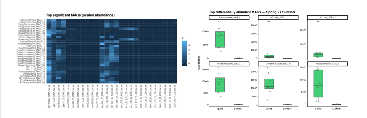
Step 9 — Boxplots of top MAGs
top_mags <- head(sig_season$MAG, 6)

plot_df <- as.data.frame(mag_t[, top_mags])
plot_df$Season <- Season
plot_long <- pivot_longer(plot_df, -Season,
                           names_to = "MAG", values_to = "Abundance")

p_box <- ggplot(plot_long, aes(x = Season, y = Abundance, fill = Season)) +
  geom_boxplot(width = 0.5, outlier.shape = 21,
               outlier.size = 1.5, alpha = 0.85) +
  geom_jitter(width = 0.1, size = 1.5, alpha = 0.5, colour = "grey30") +
  scale_fill_manual(values = c("Spring" = "#22c55e", "Summer" = "#ef4444")) +
  facet_wrap(~ MAG, scales = "free_y", ncol = 3) +
  labs(x = NULL, y = "Abundance",
       title = "Top differentially abundant MAGs — Spring vs Summer") +
  theme_classic(base_size = 11) +
  theme(legend.position = "none",
        strip.text = element_text(face = "italic", size = 8),
        plot.title = element_text(face = "bold"))

print(p_box)
Step 10 — Save combined figure
combined <- p_volcano / p_box +
  plot_annotation(tag_levels = "A")

ggsave("figures/day4_nonparametric_figure.tiff",
       combined, width = 12, height = 10,
       dpi = 300, compression = "lzw")
⚠️ Common Mistakes
Mistake 1: Using a t-test on MAG abundance data. The most common mistake in the field. MAG abundances are zero-inflated, right-skewed, and compositional. The t-test’s normality assumption is violated. Use Wilcoxon. Every time.
Mistake 2: Reporting raw p-values across 61 MAGs. With 61 tests at α = 0.05, you expect ~3 false positives by chance. Always apply p.adjust(..., method = "BH") and report adjusted p-values. This is not optional.
Mistake 3: Reporting p-values without effect sizes. A MAG with q = 0.001 and Cliff’s δ = 0.12 (negligible effect) is statistically significant but biologically irrelevant. Always pair your p-value with Cliff’s delta and its magnitude category.
Mistake 4: Not visualising before testing. Always plot distributions before running the test. A quick boxplot reveals if the “significant” difference is driven by a single outlier, which the test statistic alone will not tell you.
Mistake 5: Treating non-significant as “no difference”. With only 8 Spring samples, power is limited. Non-significant means “insufficient evidence” — not “proven identical.” Report effect sizes even for non-significant results.
Mistake 6: Forgetting exact = FALSE with ties. Microbiome data has many zeros — ties in the rank matrix. Always set exact = FALSE in wilcox.test() to avoid errors or unreliable exact p-values.
🧭 Key Takeaways
- Wilcoxon rank-sum is the correct test for two-group comparisons of MAG abundances — not the t-test, which requires normality that microbiome data never satisfies.
- Kruskal-Wallis extends to three or more groups, followed by post-hoc pairwise Wilcoxon with FDR correction.
- FDR correction (BH method) is mandatory when testing 61 MAGs simultaneously — without it, your results contain an unknown number of false positives.
- Cliff’s delta is the effect size for Wilcoxon — always report it alongside your p-value. A result without effect size is scientifically incomplete.
- Volcano plots combine effect size and significance into a single, standard visualisation for differential abundance analysis.
- Non-parametric tests and PERMANOVA answer complementary questions: PERMANOVA asks “do communities differ overall?”, Wilcoxon asks “which specific MAGs differ, and by how much?”
🔗 What’s Next
Tomorrow on Day 5, we move from group comparisons to regression — asking not just “which MAGs differ between groups” but “how does a specific MAG’s abundance change continuously with Salinity, Temperature, or ChlA?” Linear models for MAG abundance, model diagnostics, and biological interpretation of regression coefficients.
All R code and data: github.com/jojyjohn28/microbiome_stats
Found this useful? Share it with someone learning microbiome statistics.