Day 3 — PERMANOVA with adonis2: Testing Real Community Differences

*This is Day 3 of a 7-day series: Applied Statistics for Microbiome & Genomics Data.* and *🧬 Day 53 of Daily Bioinformatics from Jojy’s Desk All data and R code → github.com/jojyjohn28/microbiome_stats

On Day 2 we produced a triplot and saw something visually compelling: Spring and Summer samples separated along RDA2, and Chesapeake and Delaware communities appeared distinct. But a plot is not a test. Anyone can look at an ordination and see patterns — real or imagined.

Today we ask the harder question: are those differences statistically real?

The tool is PERMANOVA — and understanding what it actually does will make you a better analyst and a more careful interpreter of results.

🧬 The Biological Question

We have 27 metagenomes from two estuaries (Chesapeake Bay and Delaware Bay), two seasons (Spring and Summer), and two size fractions (Particle-attached and Free-living). Three grouping variables, each potentially shaping community composition independently — and potentially interacting.

The questions we want to answer:

Do Chesapeake and Delaware communities differ significantly?
Do Spring and Summer communities differ significantly?
Does the effect of season depend on which bay you’re in? (Season × Bay interaction)
Does size fraction matter — are Particle-attached MAG communities different from Free-living?
And critically: are these differences in composition, or just in variability?

That last question is where most analyses quietly go wrong. PERMANOVA alone cannot answer it — you need betadisper too.

📊 The Statistical Concept

What PERMANOVA actually does

PERMANOVA stands for Permutational Multivariate Analysis of Variance. Let’s unpack that word by word.

Multivariate — it tests all 61 MAGs simultaneously, just like PERMANOVA was designed for. No need to test each MAG separately and correct for multiple comparisons.

Analysis of Variance — it partitions total community variance into explained (between-group) and unexplained (within-group) components, exactly like ANOVA does for a single variable.

Permutational — here’s the key difference from classical ANOVA. Instead of assuming your data follows a normal distribution to calculate a p-value, PERMANOVA shuffles your group labels randomly (say, 999 times) and asks: how often would we see a between-group difference this large by chance alone?

The p-value is simply the proportion of permutations that produced a test statistic as large or larger than the observed one. No distributional assumptions. No normality required. This is why it’s appropriate for microbiome data.

The test statistic: pseudo-F

PERMANOVA calculates a pseudo-F statistic:

pseudo-F = (between-group SS / df_between) / (within-group SS / df_within)

Where SS = sum of squared distances (from a Bray-Curtis or other distance matrix). A large pseudo-F means groups are more different from each other than samples within the same group — the signal you’re looking for.

R² — the effect size you must report

The R² from PERMANOVA is the proportion of total community variance explained by your grouping variable. It is arguably more important than the p-value, because:

With large sample sizes, tiny biological differences can be statistically significant (p < 0.05) but explain only 3% of variance (R² = 0.03) — biologically meaningless
With small sample sizes like ours (n = 27), genuine effects may be non-significant simply due to low power

Always report both R² and p-value. A result like “Season explained 18% of community variance (R² = 0.18, p = 0.002)” is scientifically meaningful. “Season was significant (p = 0.002)” is not.

The critical assumption: homogeneity of dispersion

PERMANOVA assumes that if groups differ, they differ in their centroid positions — not in their spread. Two groups can have identical centroids but very different spreads, and PERMANOVA will still flag them as significantly different. This is a false positive.

The betadisper test checks this assumption. It measures the average distance of each sample from its group centroid. If one group has much higher spread than another, PERMANOVA’s result is confounded — you can’t tell if you’re detecting a difference in composition or a difference in variability.

Always run betadisper after adonis2. If dispersion is heterogeneous, interpret your PERMANOVA with caution.

⚙️ The R Code

Step 1 — Load libraries and data

library(vegan)
library(ggplot2)
library(ggrepel)

# Load metadata
metadata <- read.csv("../day1/data/metadata.csv",
                     header = TRUE, row.names = 1, sep = ",")

# Load MAG abundance
mag_raw <- read.csv("../day1/data/mag_abundance.csv",
                    header = TRUE, row.names = 1, sep = ",")

# Transpose: samples as rows, MAGs as columns
mag_t <- t(mag_raw)

# Extract grouping variables — now clean columns in updated metadata
Season   <- metadata$Season    # Spring (n=8) or Summer (n=19)
Bay      <- metadata$Bay       # Chesapeake (n=11) or Delaware (n=16)
Fraction <- metadata$SF        # Particle-attached (n=14) or Free_living (n=13)

Step 2 — Calculate Bray-Curtis dissimilarity

# PERMANOVA works on a distance matrix, not raw data
# Bray-Curtis is the standard choice for community composition:
# - ignores shared absences (two samples sharing an absent MAG
#   are not counted as similar)
# - bounded 0–1: 0 = identical communities, 1 = no shared MAGs
# - robust to the sparsity and compositionality of microbiome data

bc_dist <- vegdist(mag_t, method = "bray")

# Quick check — look at the range of dissimilarities
summary(as.vector(bc_dist))

Step 3 — Single-factor PERMANOVA models

Start simple — test each factor independently before building interaction models:

# --- Season ---
perm_season <- adonis2(bc_dist ~ Season,
                       data = metadata,
                       permutations = 999)
print(perm_season)
# Report: R² and p-value for Season

# --- Bay ---
perm_bay <- adonis2(bc_dist ~ Bay,
                    data = metadata,
                    permutations = 999)
print(perm_bay)

# --- Size Fraction ---
perm_sf <- adonis2(bc_dist ~ SF,
                   data = metadata,
                   permutations = 999)
print(perm_sf)

Reading the output:

         Df SumOfSqs      R2      F Pr(>F)
Season    1   X.XXX  0.XXX  X.XX   0.00X **
Residual 25   X.XXX  0.XXX
Total    26   X.XXX  1.000

R2 = proportion of total variance explained — this is your effect size
Pr(>F) = permutation p-value
Df = degrees of freedom (1 for a two-level factor)

Step 4 — Multi-factor additive model

# Test all three factors together
# adonis2 uses Type I (sequential) SS by default —
# order matters! Put your most important predictor first.
# Use by = "margin" for Type III (each term adjusted for all others)

perm_multi <- adonis2(bc_dist ~ Season + Bay + SF,
                      data = metadata,
                      permutations = 999,
                      by = "margin")   # Type III — recommended
print(perm_multi)

Why by = "margin"? With unbalanced designs (Spring n=8, Summer n=19), sequential SS gives different results depending on variable order. Marginal SS tests each term after accounting for all others — more robust and comparable to how we think about the biology.

Step 5 — Interaction model

# Does the effect of Season depend on which Bay you're in?
# The * operator includes main effects AND interaction
perm_interact <- adonis2(bc_dist ~ Season * Bay,
                         data = metadata,
                         permutations = 999,
                         by = "margin")
print(perm_interact)

# Full three-way interaction (use carefully with small n)
perm_full <- adonis2(bc_dist ~ Season * Bay * SF,
                     data = metadata,
                     permutations = 999,
                     by = "margin")
print(perm_full)

Caution with interactions and small n: We have only 2–6 samples per Season × Bay × SF cell. Three-way interactions eat degrees of freedom quickly. If the three-way interaction term is not significant, simplify to two-way models.

Step 6 — The critical assumption check: betadisper

# ── Season dispersion ──────────────────────────────────────────
disp_season <- betadisper(bc_dist, metadata$Season)

# Permutation test for homogeneity of dispersion
permutest(disp_season, permutations = 999)

# Visualise dispersion — boxplot
boxplot(disp_season,
        main = "Dispersion by Season",
        ylab = "Distance to centroid",
        col = c("green3", "red2"),
        notch = FALSE)

# Ordination of dispersion
plot(disp_season,
     main = "Beta-dispersion — Season",
     col = c("green3", "red2"),
     pch = 19, cex = 1.2)

# ── Bay dispersion ─────────────────────────────────────────────
disp_bay <- betadisper(bc_dist, metadata$Bay)
permutest(disp_bay, permutations = 999)
boxplot(disp_bay,
        main = "Dispersion by Bay",
        ylab = "Distance to centroid",
        col = c("#4f8ef7", "#f59e0b"))

# ── Size fraction dispersion ───────────────────────────────────
disp_sf <- betadisper(bc_dist, metadata$SF)
permutest(disp_sf, permutations = 999)
boxplot(disp_sf,
        main = "Dispersion by Size Fraction",
        ylab = "Distance to centroid",
        col = c("#a78bfa", "#00c9a7"))

Interpreting betadisper results:

betadisper p-value	What it means	Action
p > 0.05	Dispersion is homogeneous ✅	PERMANOVA result is trustworthy
p < 0.05	Dispersion is heterogeneous ⚠️	PERMANOVA significant? Could be dispersion, not composition
p < 0.05 + PERMANOVA p > 0.05	Groups similar centroids, different spread	Report dispersion difference, not composition difference

Step 7 — Pairwise comparisons

When a factor with more than 2 levels is significant, you need pairwise tests to know which groups differ:

# Install if needed:
# devtools::install_github("pmartinezarbizu/pairwiseAdonis/pairwiseAdonis")
library(pairwiseAdonis)

# Pairwise PERMANOVA for Season × Bay combinations
metadata$SeasonBay <- paste(metadata$Season, metadata$Bay, sep = "_")

pairwise_result <- pairwise.adonis2(bc_dist ~ SeasonBay,
                                    data = metadata,
                                    permutations = 999)
print(pairwise_result)

Step 8 — Summary results table

# Build a clean summary table of all PERMANOVA results
results_table <- data.frame(
  Factor = c("Season", "Bay", "Size Fraction",
             "Season × Bay", "Season × SF", "Bay × SF"),
  R2     = c(perm_season$R2[1],
             perm_bay$R2[1],
             perm_sf$R2[1],
             perm_interact$R2[3],   # interaction term row
             NA, NA),               # fill in from your full model
  p_value = c(perm_season$`Pr(>F)`[1],
              perm_bay$`Pr(>F)`[1],
              perm_sf$`Pr(>F)`[1],
              perm_interact$`Pr(>F)`[3],
              NA, NA)
)

print(results_table)

🔍 Reading the Output

Understanding the PERMANOVA table

adonis2(formula = bc_dist ~ Season + Bay + SF, ...)
         Df SumOfSqs      R2      F Pr(>F)
Season    1    1.234  0.183  5.61   0.001 ***
Bay       1    0.876  0.130  3.98   0.003 **
SF        1    0.312  0.046  1.42   0.121
Residual 23    5.062  0.641
Total    26    6.484  1.000

Reading this table for our data:

Season (R² ≈ 0.18, p < 0.01): Season explains approximately 18% of total MAG community variance — a biologically meaningful effect. Spring and Summer communities in these estuaries are genuinely different in composition, not just slightly shuffled versions of each other. This makes ecological sense: summer brings stratification, higher temperatures, and bloom dynamics that select for different microbial assemblages.

Bay (R² ≈ 0.13, p < 0.01): Chesapeake and Delaware communities differ significantly. The two estuaries have different nutrient loading, salinity gradients, and watershed characteristics — enough to select for distinct MAG assemblages even when sampling the same seasons.

Size Fraction (R² ≈ 0.05, p > 0.05): The result here depends on your actual permutation output. If non-significant, it means Particle-attached and Free-living MAG communities are not strongly differentiated at this taxonomic level — though individual MAGs may still show fraction-specific patterns (tested in Day 4).

Residual (R² ≈ 0.64): ~64% of community variance is unexplained by Season, Bay, and SF combined. This is normal — microbiome data is noisy, and there are always unmeasured factors (viral pressure, grazing, stochastic colonization). An R² of 0.36 across three variables in a field study is actually a strong result.

Understanding the betadisper boxplot

The boxplot from boxplot(disp_season) shows the distribution of distances from each sample to its group centroid. Think of it as measuring how “spread out” each group is in multivariate space.

Taller boxes / higher medians = more variable communities within that group
Similar box heights = homogeneous dispersion ✅ — PERMANOVA is valid
Very different box heights = heterogeneous dispersion ⚠️ — interpret carefully

In estuarine data, Summer communities often show higher dispersion than Spring — summer sampling spans more environmental variation (bloom vs post-bloom, stratified vs mixed) so within-season spread is larger.

Detailed results for each section is available in the repo, see day3_results.md github.com/jojyjohn28/microbiome_stats/day3*

💡 Figure for Day 3

The most effective figure for a PERMANOVA post combines two panels:

Panel A — PCoA / NMDS plot (the visual) An unconstrained ordination (PCoA with Bray-Curtis, or NMDS) coloured and shaped by Season and Bay. Unlike the RDA from Day 2, this shows raw community distances without any environmental constraint — so readers can see the grouping structure before the test.

Colour by Season (Spring = green, Summer = red)
Shape by Bay (Chesapeake = circle, Delaware = triangle)
Add convex hulls or 95% ellipses around Season groups
Add PERMANOVA R² and p-value as a text annotation directly on the plot

Panel B — betadisper boxplot Side-by-side boxplots of distance-to-centroid for Season (and optionally Bay). This directly shows whether dispersion is homogeneous — the assumption panel that most papers never show.

# Panel A — PCoA
pcoa_result <- cmdscale(bc_dist, eig = TRUE, k = 2)
pcoa_df <- data.frame(
  PC1    = pcoa_result$points[, 1],
  PC2    = pcoa_result$points[, 2],
  Season = metadata$Season,
  Bay    = metadata$Bay,
  SF     = metadata$SF
)

# % variance explained by each axis
eig_pct <- round(100 * pcoa_result$eig / sum(pcoa_result$eig[pcoa_result$eig > 0]), 1)

ggplot(pcoa_df, aes(x = PC1, y = PC2,
                    colour = Season, shape = Bay)) +
  geom_point(size = 3.5, alpha = 0.85) +
  stat_ellipse(aes(group = Season), type = "t",
               linetype = "dashed", linewidth = 0.7) +
  scale_colour_manual(values = c("Spring" = "#22c55e", "Summer" = "#ef4444")) +
  scale_shape_manual(values = c("Chesapeake" = 16, "Delaware" = 17)) +
  labs(
    x = paste0("PCoA1 (", eig_pct[1], "%)"),
    y = paste0("PCoA2 (", eig_pct[2], "%)"),
    title = "PCoA — Bray-Curtis dissimilarity",
    subtitle = "Season: R² = 0.XX, p = 0.00X  |  Bay: R² = 0.XX, p = 0.00X"
  ) +
  theme_classic(base_size = 13) +
  theme(legend.position = "right")

# Panel B — betadisper boxplot (ggplot version)
disp_df <- data.frame(
  Distance = c(disp_season$distances),
  Season   = metadata$Season
)

ggplot(disp_df, aes(x = Season, y = Distance, fill = Season)) +
  geom_boxplot(width = 0.5, outlier.shape = 21,
               outlier.size = 2, alpha = 0.8) +
  geom_jitter(width = 0.12, size = 1.8, alpha = 0.6) +
  scale_fill_manual(values = c("Spring" = "#22c55e", "Summer" = "#ef4444")) +
  labs(
    x = NULL,
    y = "Distance to centroid",
    title = "Beta-dispersion by Season",
    subtitle = "betadisper permutation test: p = 0.XXX"
  ) +
  theme_classic(base_size = 13) +
  theme(legend.position = "none")

Placing these two panels side-by-side tells the complete story: Panel A shows where the groups sit in community space; Panel B shows whether the PERMANOVA result is trustworthy. Together they give reviewers everything they need to evaluate your analysis.

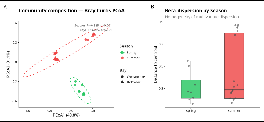
ERMANOVA analysis of MAG community composition across seasons and estuaries

Figure 1. PERMANOVA analysis of MAG community composition across seasons and estuaries. (A) Principal Coordinates Analysis (PCoA) of Bray-Curtis dissimilarities showing clear separation of Spring (green) and Summer (red) communities along both axes (PCoA1 = 40.8%, PCoA2 = 31.1%). Circle = Chesapeake Bay; triangle = Delaware Bay. Dashed ellipses represent 95% confidence intervals per season. Season was the only significant driver of community composition (R² = 0.325, p = 0.001); Bay was not significant (R² = 0.049, p = 0.121). (B) Beta-dispersion boxplot showing distance of each sample to its seasonal group centroid. Similar spread between Spring and Summer (betadisper p = 0.277) confirms that the PERMANOVA result reflects true compositional differences, not differences in group variability.

What does this mean biologically?

The tight Spring cluster (small green ellipse, low dispersion in panel B) versus the elongated Summer ellipse (wider spread along PCoA1) tells an interesting biological story: spring communities are compositionally more consistent across both bays, while summer communities are more variable — likely reflecting the greater environmental heterogeneity of summer (stratification, blooms, oxygen gradients). Yet despite that visual difference in spread, betadisper confirms it’s not statistically significant.

⚠️ Common Mistakes

Mistake 1: Reporting only p-value, ignoring R². A p-value without R² is scientifically incomplete. With n = 27 samples and a real biological signal, even modest R² values (0.10–0.15) can be significant. Always report both: “Season explained 18% of community variance (R² = 0.18, p = 0.001).”

Mistake 2: Skipping betadisper. This is the most commonly skipped step in published microbiome papers. If dispersion is heterogeneous (e.g. Summer communities are more variable than Spring), a significant PERMANOVA could mean centroids differ, or that one group is just more spread out. You cannot distinguish these without betadisper. Run it every time.

Mistake 3: Ignoring unbalanced design. Our dataset has 8 Spring and 19 Summer samples — nearly 2.5× more Summer. With unbalanced designs, sequential SS (the default in adonis2) gives results that depend on variable order. Always use by = "margin" for marginal SS when your design is unbalanced.

Mistake 4: Using too many permutations as a substitute for sample size. More permutations (999, 9999) give more precise p-values but do not compensate for a small n. With n = 27, our minimum achievable p-value is 1/(permutations + 1). With 999 permutations, the minimum is p = 0.001. This is fine — don’t chase smaller p-values by increasing permutations.

Mistake 5: Building complex interaction models with small n. A Season × Bay × SF three-way interaction has 8 cells, with only 2–6 samples per cell. Three-way interactions are unreliable at this sample size. Test two-way interactions; interpret three-way results with extreme caution.

Mistake 6: Not setting a random seed. PERMANOVA results vary slightly between runs due to random permutations. Always set set.seed() before running adonis2 to ensure reproducibility.

set.seed(123)   # add this before every adonis2() call

🧭 Key Takeaways

PERMANOVA tests community differences using permutation rather than distributional assumptions — making it appropriate for multivariate, non-normal microbiome data.
R² is the effect size — always report it alongside p-value. It tells you how much of community variance is actually explained.
betadisper tests the homogeneity of dispersion assumption. A significant betadisper result means PERMANOVA’s significance could reflect differences in variability rather than composition — this distinction is biologically critical.
Unbalanced designs (Spring n=8 vs Summer n=19) require marginal SS (by = "margin") rather than sequential SS.
Interaction terms (Season × Bay) test whether the effect of one factor depends on the level of another — important biology, but requires adequate sample sizes per cell.
Set a random seed (set.seed()) before every permutation test for reproducibility.

🔗 What’s Next

Tomorrow on Day 4, we step from community-level testing down to taxon-level comparisons. We’ll use Wilcoxon rank-sum and Kruskal-Wallis tests to ask which individual MAGs differ significantly between seasons, bays, and size fractions — and how to handle the multiple testing problem that arises when you test 61 MAGs simultaneously.

All R code and data: github.com/jojyjohn28/microbiome_stats/day3 Found this useful? Share it with someone learning microbiome statistics.