Whole Genome Sequencing — Day 5: Comparative & Downstream Genomic Analyses
🧬 Whole Genome Sequencing — Day 5
Comparative & Downstream Genomic Analyses 👉In Day 1, we cleaned raw reads. 👉In Day 2, we assembled genomes and evaluated quality. 👉In Day 3, we placed genomes in taxonomic and phylogenetic context. 👉In Day 4, we annotated genomes and identified functional potential.
Today, in Day 5, we shift from individual genomes to comparative insights: How do genomes differ? What unique functions do they encode? What risks or opportunities do they present? This step transforms genome collections into ecological and biotechnological insights by comparing gene content, identifying biosynthetic potential, and screening for clinically relevant features.
🎯 Goal of Day 3
PMove from single genomes to comparative and ecological insights Specifically, we aim to: ✔ Define core and accessory genomes across collections ✔ Identify secondary metabolite biosynthetic gene clusters ✔ Screen for antimicrobial resistance and virulence factors ✔ Detect and characterize plasmids ✔ Validate genome topology and circularization This workflow scales from small genome sets to hundreds of isolates or MAGs.
🧪 Comparative Genomics Strategy
Comparative analyses work best when structured around specific biological questions:
| Analysis | Question |
|---|---|
| Pangenome analysis | What genes are shared vs. strain-specific? |
| Secondary metabolite screening | What biosynthetic potential exists? |
| Pathogen screening | Are there AMR genes or virulence factors? |
| Plasmid detection | What mobile genetic elements are present? |
| Topology validation | Are genomes complete and circularized? |
🧠 Why Comparative Genomics Matters
Individual genomes tell us what one organism can do.
Comparative genomics reveals: ● Functional diversity within populations
● Evolutionary adaptation strategies
● Horizontal gene transfer and mobile elements
● Biotechnological potential (enzymes, metabolites)
● Public health risks (AMR, virulence)
Comparative genomics is essential for: ● Understanding strain-level variation ● Identifying biomarkers or diagnostic targets ● Prioritizing genomes for downstream work ● Linking genomic diversity to ecological roles
🧰 Tools Used in Day 5
🔹 PanX Pangenome analysis and visualization 🔹 antiSMASH Secondary metabolite biosynthetic gene cluster prediction 🔹 BiG-SCAPE Biosynthetic gene cluster similarity networks 🔹 Abricate Rapid screening for AMR genes, virulence factors, and plasmids 🔹 Plsdb / PlasmidFinder Plasmid detection and characterization 🔹 PLSMER Machine learning-based plasmid sequence identification 🔹 SPAdes (plasmidSPAdes mode) Targeted plasmid assembly 🔹 SnapGene / Geneious Plasmid visualization and annotation Each tool addresses a different dimension of comparative and applied genomics.
🧬 Step 1: Pangenome Analysis with PanX
Pangenome analysis partitions genes into: ● Core genome – genes present in all strains ● Accessory genome – genes present in some strains ● Unique genes – strain-specific genes This reveals functional diversity, niche adaptation, and horizontal gene transfer.
For more deatails about PanX from installation to run please visit : https://jojyjohn28.github.io/blog/panx-pangenome-analysis/
You can always Extract Core and Pan Genes Without Visualization using custom Python Script. Please see core_pan_from_list.py , inside https://github.com/jojyjohn28/whole-genome-sequencing-analysis/day5
What PanX Tells Us ✔ Which genes are universally conserved (core metabolism) ✔ Which genes are variable (niche-specific functions) ✔ Gene gain/loss patterns across phylogeny ✔ Functional stratification within populations Pangenomes are especially powerful when combined with Day 3 phylogenies and Day 4 functional annotations.
🧬 Step 2: Secondary Metabolite Screening with antiSMASH
Secondary metabolites include antibiotics, toxins, pigments, and signaling molecules. Many are encoded by biosynthetic gene clusters (BGCs). antiSMASH predicts BGCs and compares them to known compounds.
# Install antiSMASH via conda
conda install -c bioconda antismash
Running antiSMASH
antismash genome.gbk \
  --output-dir antismash_out \
  --genefinding-tool prodigal \
  --cpus 16
If it is 1 genome or few genomes and you are not experienced to run the stand-alone version, antiSMASH is available as web based platform. Please visit :https://antismash.secondarymetabolites.org/#!/start 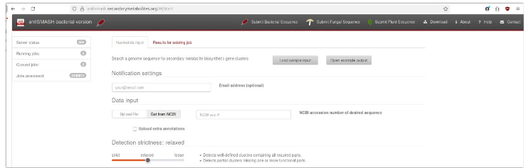
Key Outputs
● HTML report with interactive BGC visualization
● GenBank files with annotated BGCs
● Predicted compound classes (NRPS, PKS, terpene, etc.)
What antiSMASH Reveals ✔ Biosynthetic potential for novel metabolites ✔ Known BGCs with compound matches ✔ Evolutionary conservation of BGCs across strains
🧬 Step 3: BGC Similarity Networks with BiG-SCAPE
When you have many genomes, BiG-SCAPE clusters similar BGCs into gene cluster families (GCFs). This enables: ● Cross-genome BGC comparison ● Identification of conserved vs. unique BGCs ● Prioritization of novel clusters
Installation
# Install BiG-SCAPE
conda install -c bioconda bigscape
Running BiG-SCAPE
bigscape -i antismash_out/ \
  -o bigscape_out \
  --pfam_dir /path/to/pfam \
  --mode auto \
  --cutoffs 0.3 0.5 0.7
Key Outputs
● Network diagrams of BGC families
● GCF assignments for each genome
● Distance matrices for comparative analysis
BiG-SCAPE + antiSMASH together provide a genome-scale view of biosynthetic diversity. 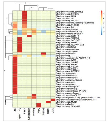
This figure shows a new starin of Streptomyces SOSIST-3 isolated from Southern Oceans, the manuscript is accepted in Molecular biology Reports. More details see : https://jojyjohn28.github.io/collaborations/ and https://jojyjohn28.github.io/publications/
🧬 Step 4: Pathogen Screening with Abricate
Whole genomes are typically screened against two different types of databases to assess their pathogenic potential: i ARGs (Antibiotic Resistance Genes) iiVirulence genes
Tool: Abricate
Abricate (https://github.com/tseemann/abricate) is a mass screening tool that rapidly identifies antimicrobial resistance and virulence genes by BLAST against multiple curated databases.
Available Databases in Abricate
Abricate supports the following databases:
● NCBI – NCBI Bacterial Antimicrobial Resistance Reference Gene Database
● CARD – Comprehensive Antibiotic Resistance Database
● ARG-ANNOT – Antibiotic Resistance Gene-ANNOTation
● ResFinder – Acquired antimicrobial resistance genes
● MEGARES – MEGARes resistance database
● EcOH – E. coli virulence genes
● PlasmidFinder – Plasmid replicons
● Ecoli_VF – E. coli virulence factors
● VFDB – Virulence Factor Database
Database Selection Strategy
For comprehensive screening, use the following databases:
For ARGs (Antibiotic Resistance Genes): ● ARG-ANNOT ● CARD ● ResFinder
For Virulence Genes: ● VFDB (Virulence Factor Database)
Installation
conda install -c bioconda abricate
Running Abricate
*Screen for ARGs
# Using CARD database
abricate --db card genome.fasta > genome_card.tab

# Using ResFinder database
abricate --db resfinder genome.fasta > genome_resfinder.tab

# Using ARG-ANNOT database
abricate --db argannot genome.fasta > genome_argannot.tab
*Screen for Virulence Factors
# Using VFDB database
abricate --db vfdb genome.fasta > genome_vfdb.tab
*Screen for Plasmid Replicons
abricate --db plasmidfinder genome.fasta > genome_plasmids.tab
Scaling to Multiple Genomes
# Batch screening for ARGs (CARD example)
for genome in *.fasta; do
  abricate --db card $genome > ${genome%.fasta}_card.tab
done

# Batch screening for virulence factors
for genome in *.fasta; do
  abricate --db vfdb $genome > ${genome%.fasta}_vfdb.tab
done

# Summarize results across all genomes
abricate --summary *_card.tab > card_summary.tab
abricate --summary *_vfdb.tab > vfdb_summary.tab
Comprehensive Screening Workflow For complete pathogen characterization, screen each genome against all relevant databases. An example bash script (comp_screening.sh) is included in https://github.com/jojyjohn28/whole-genome-sequencing-analysis/day5
What Abricate Provides ✔ Presence/absence of resistance genes across multiple databases ✔ Virulence factor distribution and identification ✔ Plasmid-associated gene detection ✔ Gene coverage and identity statistics ✔ Rapid, scalable screening for large datasets
Using multiple databases (CARD, ResFinder, ARG-ANNOT) for ARG screening ensures comprehensive detection, as different databases may capture different resistance mechanisms or gene variants.
🧬 Step 5: Plasmid Detection & Characterization
Plasmids carry mobile genes involved in: ● Antibiotic resistance ● Virulence ● Metabolic versatility ● Horizontal gene transfer
Detecting and characterizing plasmids helps us understand genome plasticity and ecological adaptation. Tools for Plasmid Detection 🔹 Plasmer – plasmid identification 🔹 PlasmidFinder – Database-based replicon detection 🔹 Prokka – Annotates plasmid sequences 🔹 SPAdes (plasmidSPAdes mode) – Assembles plasmids from raw reads 🔹 SnapGene / Geneious – Visualizes and annotates plasmid maps
a. Plasmid Identification with Plasmer Plasmer uses machine learning to classify sequences as chromosomal or plasmid-derived. GitHub: https://github.com/nekokoe/Plasmer
Installation Option 1: Using Conda (Recommended)
conda install -c iskoldt -c bioconda -c conda-forge -c defaults plasmer
Running Plasmer
Plasmer -g input.fasta \
  -p output_prefix \
  -d /path/to/plasmer_db \
  -t 16 \
  -m 500 \
  -l 500000 \
  -o output_directory
Key Parameters
-g –genome Input fasta file [required] -p –prefix Prefix for output files [Default: output] -d –db Path to Plasmer databases [required] -t –threads Number of threads [Default: 8] -m –minimum_length Minimum sequence length (bp) [Default: 500] -l –length Chromosome length threshold (bp) [Default: 500000] -o –outpath Output directory [required]
What Plasmer Provides ✔ Plasmid vs. chromosome classification ✔ Machine learning-based prediction ✔ Suitable for draft assemblies with multiple contigs
b. Plasmid Replicon Detection with PlasmidFinder PlasmidFinder identifies plasmid replicons via BLAST against a curated database.
Installation
conda install -c bioconda plasmidfinder
Running PlasmidFinder
plasmidfinder.py -i genome.fasta -o plasmidfinder_out -p /path/to/plasmidfinder_db
c. Plasmid Assembly with SPAdes If plasmids are present in raw sequencing data, plasmidSPAdes can assemble them separately. Running plasmidSPAdes
spades.py --plasmid \
  -1 reads_R1.fastq.gz \
  -2 reads_R2.fastq.gz \
  -o plasmid_assembly \
  -t 16
Key Output ● plasmids.fasta → assembled plasmid sequences
d. Plasmid Annotation with Prokka Once plasmids are assembled or extracted, annotate them with Prokka.
prokka plasmid.fasta \
  --outdir plasmid_annotation \
  --prefix plasmid \
  --compliant
e. Plasmid Visualization with SnapGene For circular plasmid maps and publication-quality figures:
● Import annotated GenBank file into SnapGene ● Add features (AMR genes, replicons, origins) ● Export circular map as PNG or SVG
Alternative: Use Geneious or custom scripts with biopython and matplotlib.
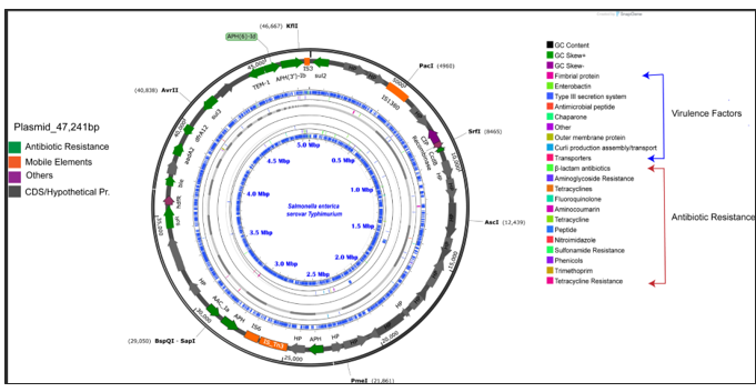
The image shows a multidrug plasmid annotated with a whole genome of *Salmonella sp.
🧬 Step 6: Genome Circularization & Topology Validation
Complete genomes should be: ● Circularized – chromosomes form closed loops
● Topology-validated – no misassemblies or chimeric joins
This is especially important for:
● Plasmid characterization
● Complete reference genomes
● Comparing assembly quality
Tools for Topology Validation 🔹 Unicycler – Includes circularization detection 🔹 CheckM / CheckM2 – Flags genome completeness issues 🔹 Bandage – Visualizes assembly graphs 🔹 Custom scripts – Check for overlapping contig termini
For more details please see:https://jojyjohn28.github.io/blog/genome-topology-and-genome-report/
📊 Scaling Comparative Analyses to 100+ Genomes
For large genome collections: ✔ Use PanX for genome-wide gene presence/absence ✔ Run antiSMASH + BiG-SCAPE for biosynthetic diversity ✔ Screen all genomes with Abricate for AMR/virulence ✔ Detect plasmids with PLSMER + PlasmidFinder ✔ Aggregate results into summary tables or heatmaps This enables: ● Functional trait mapping onto phylogenies ● Identification of high-risk or high-value strains ● Comparative metabolic and biosynthetic potential
🧠 Key Takeaways from Day 5
● Pangenome analysis reveals core vs. variable gene content ● antiSMASH identifies biosynthetic potential for novel compounds ● Abricate rapidly screens for AMR, virulence, and plasmids ● Plasmid detection and characterization reveal mobile genetic elements ● Topology validation ensures genome completeness ● Comparative genomics bridges sequence data and biological insight
🔜 What’s Next?
With comparative and functional analyses complete, you now have: ● Annotated, taxonomically placed genomes ● Functional trait distributions ● AMR and biosynthetic potential ● Pangenome structure These datasets can be integrated with: ● Metagenomics (for community-level insights) ● Transcriptomics (for gene expression validation) ● Metabolomics (for linking genes to metabolites) ● Ecological metadata (for trait-environment correlations)
All codes can be found at day 5 of : https://github.com/jojyjohn28/whole-genome-sequencing-analysis