🧬 Whole Genome Sequencing — Day 4

Genome Annotation & Functional Potential

👉In Day 1, we cleaned raw reads. 👉In Day 2, we assembled genomes and evaluated quality and topology. 👉In Day 3, we placed genomes in a taxonomic and phylogenetic context.

Today, in Day 4, we answer the most biologically meaningful question:

What can this genome actually do?

This step transforms assembled genomes into functional blueprints by identifying genes, protein domains, pathways, and metabolic capabilities.

🎯 Goal of Day 4

Identify genes, pathways, and metabolic potential encoded in genomes

Specifically, we aim to:

✔ Predict protein-coding genes ✔ Assign functional annotations ✔ Reconstruct metabolic pathways ✔ Compare functional potential across many genomes

This workflow is designed for isolate genomes and MAG collections, and scales cleanly to hundreds of genomes.

🧪 Annotation Strategy: A Layered Approach

Genome annotation works best when done in layers, each answering a different question: | Layer | Question | | —————— | —————————————- | | Gene prediction | Where are the genes? | | Rapid annotation | What are they likely doing? | | Domain annotation | What conserved functions do they encode? | | Pathway annotation | How do genes connect into metabolism? | | Trait screening | What ecological traits are present? |

🧠 Why Genome Annotation Matters

A genome sequence without annotation is just a long string of nucleotides.

Genome annotation enables us to:

● Interpret ecological strategies

● Predict metabolic roles

● Identify functional redundancy or specialization

● Link taxonomy to ecosystem function

● Good annotation is the foundation for:

● Comparative genomics

● Metabolic modeling

● Transcriptomic integration

● Functional redundancy analyses

🧪 Annotation Strategy Overview

Genome annotation is best approached in layers, not with a single tool.

Layered annotation strategy used here:

1️⃣ Gene prediction – Where are the genes? 2️⃣ Rapid annotation – What are they likely doing? 3️⃣ Domain-based annotation – What functional motifs do proteins contain? 4️⃣ Pathway-level reconstruction – How do genes connect into metabolism?

🧰 Tools Used in Day 4

🔹 Prokka

Rapid, genome-scale annotation pipeline for bacterial and archaeal genomes.

🔹 Prodigal

Accurate gene prediction engine used internally by many annotation tools.

🔹 InterProScan

Protein domain and motif identification across multiple databases.

🔹 DRAM

High-level metabolic and pathway-centric genome annotation.

Each tool complements the others rather than replacing them.

🧬 Step 1: Gene Prediction with Prodigal

Gene prediction identifies open reading frames (ORFs) and defines the basic gene catalog.

prodigal \
  -i genome.fasta \
  -a genome.faa \
  -d genome.fna \
  -o genome.genes.gbk \
  -p single

Key outputs

● faa → predicted proteins

● fna → nucleotide CDS

● gbk → gene coordinates

Prodigal is: ✔ Fast ✔ Accurate ✔ Well-suited for isolates and high-quality MAGs

🧬 Step 2: Rapid Genome Annotation with Prokka

Prokka wraps gene prediction and functional assignment into a single, fast pipeline.

prokka genome.fasta \
  --outdir prokka_out \
  --prefix genome \
  --cpus 16

What Prokka provides

● Gene names and product descriptions

● rRNA, tRNA, tmRNA prediction

● GFF, GenBank, and protein FASTA files

Prokka is ideal for: ✔ First-pass annotation ✔ NCBI submissions ✔ Comparative gene counts

🧬 Step 3: Protein Domain Annotation with InterProScan

While Prokka assigns gene names, InterProScan identifies conserved protein domains, which is critical for:

● Novel proteins

● Hypothetical genes

● Functional inference beyond BLAST hits

interproscan.sh \
  -i genome.faa \
  -o genome.interpro.tsv \
  -f TSV \
  -dp \
  --cpu 32

Why domain-based annotation matters

● Domains are more conserved than full-length proteins

● Enables functional inference for unknown genes

● Links proteins to GO terms and enzyme classes

🧬 Step 4: Metabolic & Pathway Annotation with DRAM

DRAM integrates multiple databases to reconstruct genome-scale metabolic potential. DRAM annotation

DRAM.py annotate \
  -i genome.fasta \
  -o dram_out \
  --threads 32

DRAM distillation (summaries)

DRAM.py distill \
  -i dram_out/annotations.tsv \
  -o dram_out/genome_summaries

DRAM excels at ✔ Central carbon metabolism ✔ Nitrogen, sulfur, hydrogen pathways ✔ CAZymes and polysaccharide utilization ✔ Transporters and redox systems

This moves annotation from gene lists → biological interpretation. 🧠 Focus Areas: Core Metabolic Pathways

DRAM distillation gives details on core metabolic potential, including:

🔹 Energy metabolism

Glycolysis

TCA cycle

Oxidative phosphorylation

Fermentation pathways

🔹 Carbon utilization

Sugar transporters

Polysaccharide degradation

Organic acid metabolism

🔹 Nitrogen & sulfur metabolism

Nitrate/nitrite reduction

Amino acid biosynthesis

Sulfur assimilation

These pathways define how organisms:

● Acquire energy

● Use resources

● Interact with their environment

📊 Scaling Annotation to 100+ Genomes

For large genome sets:

✔ Run Prokka and Prodigal in batch mode ✔ Use DRAM summaries for comparison tables ✔ Aggregate pathway presence/absence matrices ✔ Combine with Day 3 taxonomy and phylogeny

This enables:

● Functional clustering

● Ecological stratification

● Trait-based comparisons

🔍 Trait-Based Screening: From Annotation to Ecology

Once annotation is complete, we can screen genomes for specific ecological traits, such as:

● Biofilm formation

● EPS (exopolysaccharide) production

● Motility

● Stress response

● Host or particle association

This is especially powerful for comparative genomics and functional redundancy analyses.

🧬 Example 1: Screening for Biofilm-Related Genes (InterProScan)

Step 1: Create a reference keyword list

Create a simple table (CSV or Excel) with keywords or domain IDs:

Keyword
biofilm
adhesion
fimbrial
pilus
curli
polysaccharide-binding

This can also include:

● Pfam IDs

● GO terms

● InterPro IDs

Step 2: Filter InterProScan results using pandas

You can use filter.py for filtering the annotation file with reference file. All codes can be found at : https://github.com/jojyjohn28/whole-genome-sequencing-analysis This produces a genome-specific list of candidate biofilm genes.

🧬 Example 2: Screening for EPS-Related Genes (DRAM / KEGG)

DRAM outputs include KEGG IDs, CAZymes, and functional descriptions, making them ideal for EPS screening.

Step 1: Prepare a reference list

Keyword
exopolysaccharide
capsule
glycosyltransferase
alginate
cellulose
levan

🧬 Merging Functional Traits with Quantitative Data

Trait screening becomes even more powerful when merged with abundance or expression data.

A generalized version of workflow is given in /scripts as merge.py

🔑 How Keywords Are Used for Functional Screening

Many ecological traits (e.g., biofilm formation, EPS production, adhesion, motility) are not represented by a single gene, but by groups of genes, domains, or pathways. Keyword-based screening provides a flexible, transparent way to identify such traits across genomes.

Below are two common and complementary approaches.

🧭 Option 1: Build Keyword-Based References from Databases

Keywords can be translated into reference identifiers using established databases.

🔹 InterPro / Pfam (protein domains)

Use keywords on the InterPro or Pfam websites to identify relevant domains:

Examples:

● biofilm → adhesion domains, pili, fimbriae

● EPS → glycosyltransferases, polysaccharide biosynthesis proteins

You can then screen InterProScan outputs using:

● InterPro IDs

● Pfam accessions

● Domain descriptions

This approach is robust for trait-level inference, even when gene names are ambiguous.

🔹 KEGG (pathways & enzymes)

KEGG keywords can be used to identify:

● Pathway modules (e.g., polysaccharide biosynthesis)

● Enzyme classes (e.g., glycosyltransferases)

● KO identifiers linked to EPS or biofilm pathways

DRAM outputs already integrate KEGG annotations, making KEGG-based screening especially convenient.

🗂️ Option 2: Create a Keyword Filter List and Screen Locally

For large genome sets, a practical approach is to create a simple keyword reference file and use it to filter annotation outputs.

Example keyword list (trait_keywords.txt):

biofilm
adhesion
pilus
fimbrial
exopolysaccharide
capsule
glycosyltransferase
alginate
cellulose

This file can be reused across:

● InterProScan outputs

● DRAM annotations

● Prokka product descriptions

📊 Example: Keyword-Based Screening in R

You can use screening_traits.R as minimal R workflow for screening annotation tables using keywords.

What this does

● Searches annotation descriptions for any keyword match

● Returns a genome-specific list of candidate trait genes

● Scales easily to hundreds of genomes

🧠 Best Practices

● Use keywords + domain IDs when possible

● Keep keyword lists transparent and version-controlled

● Treat results as hypothesis-generating, not definitive proof

● Combine with pathway context (DRAM) and expression data when available

This keyword-driven approach bridges the gap between raw annotation tables and ecological interpretation, making it especially powerful for comparative genomics and other downstream analyses.

🧠 Key Takeaways from Day 4

● Annotation works best in layers ● Prodigal ensures accurate gene prediction ● Prokka provides rapid functional context ● InterProScan enables trait-level screening ● DRAM connects genes into metabolic pathways ● Simple keyword-based filtering can reveal powerful ecological insights

🔜 Coming Up: Day 5

Day 5 — Comparative Genomics & Functional Comparisons

We’ll integrate taxonomy (Day 3) and function (Day 4) to compare genomes across environments, clades, and ecological strategies.

All codes can be found at : https://github.com/jojyjohn28/whole-genome-sequencing-analysis

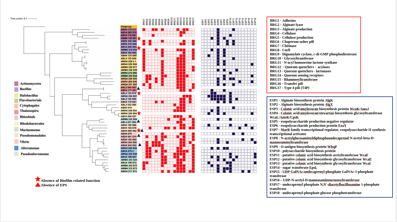
These functional screening results can be combined with genome taxonomy and phylogeny and used as annotation layers in iTOL. For example, the figure below illustrates biofilm-related gene screening across 200+ genomes, where the presence or absence of biofilm-associated traits is overlaid onto the phylogenomic tree as metadata strips or heatmaps. This integration allows rapid visualization of how functional traits are distributed across taxonomic lineages and evolutionary clades, enabling direct comparison of functional potential within and between groups.