Whole Genome Analysis — Day 1: From Raw Reads to Clean, Assembly-Ready Data
🧬 Whole Genome Analysis — Day 1
From Raw Reads to Clean, Assembly-Ready Data
Every genome project starts at the same place: raw sequencing files.
Before assembly, annotation, or comparative genomics, it is critical to confirm that the data you received is complete, uncorrupted, and of sufficient quality.
In this post, I walk through Day 1 of a whole-genome sequencing (WGS) workflow, covering both Illumina (short reads) and Oxford Nanopore (long reads).
📂 Input Data Formats
Typical WGS inputs include:
Illumina (paired-end)
sample_R1.fastq.gz
sample_R2.fastq.gz
📂 Oxford Nanopore
sample_nanopore.fastq.gz
These files often arrive from sequencing facilities or collaborators and should never be trusted blindly.
🔐 Step 0 — File Integrity Check (md5sum)
Before opening or processing FASTQ files, verify they were transferred correctly.
md5sum *.fastq.gz
Compare the output against checksums provided by the sequencing facility.
✅ Why this matters
• Prevents silent file corruption
• Saves hours of debugging downstream
• Essential for reproducible genomics
🔍 Step 1 — Quality Control of Illumina Reads (FastQC)
What is FastQC?
FastQC provides a quick visual summary of sequencing quality for FASTQ files. It works on raw or trimmed Illumina data and produces an interactive HTML report.
Installation
conda install -c bioconda fastqc
or on HPC systems you can use module load.
Run FastQC
mkdir fastqc_raw
fastqc -o fastqc_raw *.fastq.gz
🔁 Scaling FastQC for 100+ Genomes
Running FastQC on one or two samples is easy. But real projects often involve hundreds of genomes or metagenomes, each with paired-end reads.
Instead of running FastQC manually for each sample, you can automate it using either:
• a simple Bash loop (local or login node)
• a SLURM batch script (recommended for HPC environments)
🧪 Option 1 — FastQC Using a Bash Loop
This approach works well for:
• local machines
• small to medium datasets
• quick exploratory QC
✅ Advantages
• Simple
• Transparent
• Easy to debug
⚠️ Limitations
• Runs sequentially
• Not ideal for very large datasets
🖥️ Option 2 — FastQC as a SLURM Batch Job (HPC-friendly)
For large projects (100+ samples), always prefer batch execution.
⚙️ Why Batch Processing Matters
When working with large datasets, batch processing:
• avoids overloading login nodes
• scales efficiently across cores
• ensures reproducibility
• allows unattended execution
💡 Tip: Combine FastQC with MultiQC later to summarize all reports in one dashboard.
All example scripts are available in the project repository. https://github.com/jojyjohn28/whole-genome-sequencing-analysis
📊 Interpreting FastQC Reports
Key modules to inspect:
• Basic Statistics – total reads, GC %, read length
• Per Base Sequence Quality – look for quality drops at read ends
• Per Sequence Quality Scores – distribution of read quality
• Adapter Content – presence of sequencing adapters
• Overrepresented Sequences – contamination or adapters
• Sequence Duplication Levels – PCR artifacts or bias
Understanding the plot
• Red line → median quality
• Yellow box → interquartile range (25–75%)
• Whiskers → 10–90%
• Blue line → mean quality
• Green / Orange / Red background → good / warning / poor quality
📌 Raw data often looks messy — that’s normal.
See the plots below as an example to learn (source-Google)
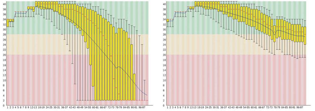
Left: Raw reads with severe quality drop toward read ends Right: Trimmed reads with stabilized base quality (These plots clearly show why trimming is required before assembly.)
If you have many genomes you can use standalone Python script that parses FastQC outputs and generates a summary table you can use for reporting, plotting, or downstream filtering. For more details please see Day 1 in https://github.com/jojyjohn28/whole-genome-sequencing-analysis look for fastqc_to_table.py and fastqc_to_table.md.
🔬 Step 2 — Quality Control of Nanopore Reads (NanoPlot)
Illumina-style QC tools are not suitable for Nanopore data.
What is NanoPlot?
NanoPlot visualizes:
• Read length distribution
• Quality vs read length
• Yield over time
• N50 / N90 statistics
Installation
conda install -c bioconda nanoplot
Run NanoPlot
NanoPlot \
  --fastq sample_nanopore.fastq.gz \
  --outdir nanoplot_results \
  --threads 8
For loop/batch script please visit the project repository (Day1). https://github.com/jojyjohn28/whole-genome-sequencing-analysis
What to look for
• Wide read length distribution (expected)
• No extreme quality collapse
• Reasonable N50 for your library type
✂️ Step 3 — Read Trimming (Illumina)
Raw Illumina reads almost always contain:
• Adapter contamination
• Low-quality bases at ends
Two commonly used tools are Trimmomatic and Cutadapt.
🔧 Trimmomatic Installation
conda install -c bioconda trimmomatic
General Default Command
trimmomatic PE -threads 16 \
  sample_R1.fastq.gz sample_R2.fastq.gz \
  sample_R1.paired.fastq.gz sample_R1.unpaired.fastq.gz \
  sample_R2.paired.fastq.gz sample_R2.unpaired.fastq.gz \
  ILLUMINACLIP:TruSeq3-PE.fa:2:30:10 \
  LEADING:3 \
  TRAILING:3 \
  SLIDINGWINDOW:4:15 \
  MINLEN:50
Key Trimming Options
• ILLUMINACLIP → adapter removal
• SLIDINGWINDOW → dynamic quality trimming
• LEADING / TRAILING → end trimming
• MINLEN → drop short reads
✂️ Cutadapt (Alternative)
Cutadapt provides more flexible adapter handling and is increasingly popular. General Default Command
cutadapt \
  -a AGATCGGAAGAGC \
  -A AGATCGGAAGAGC \
  -q 20,20 \
  -m 50 \
  -o sample_R1.trimmed.fastq.gz \
  -p sample_R2.trimmed.fastq.gz \
  sample_R1.fastq.gz sample_R2.fastq.gz
🔁 Step 4 — Post-Trimming QC
Always rerun FastQC after trimming:
You should observe:
• Cleaner base quality profiles
• Reduced adapter content
• More uniform read lengths
📁 Output of Day 1
By the end of Day 1, you should have:
Illumina:
sample_R1.trimmed.fastq.gz
sample_R2.trimmed.fastq.gz

Nanopore:
sample_nanopore.fastq.gz (QC-validated)
🧠 Why Day 1 Matters
All downstream steps assume:
• Accurate base calls
• Minimal sequencing artifacts
• Reliable read lengths
Skipping or rushing QC can:
• Break assemblies
• Inflate errors
• Bias comparative genomics
Clean input = trustworthy genomes