From QIIME 2 to R — visualizing your 16S amplicon results

🧬 𝐷𝑎𝑦 73 𝑜𝑓 𝐷𝑎𝑖𝑙𝑦 𝐵𝑖𝑜𝑖𝑛𝑓𝑜𝑟𝑚𝑎𝑡𝑖𝑐𝑠 𝑓𝑟𝑜𝑚 𝐽𝑜𝑗𝑦’𝑠

You ran your 16S samples through QIIME 2. You have feature tables, taxonomy assignments, a phylogenetic tree, and alpha and beta diversity results. You opened a few .qzv files in the browser, which is great for exploration — but when it comes to making figures for a paper, or for priliminary analysis you want full control in R.

This post is the bridge between your QIIME 2 outputs and your first set of publication-quality figures. We will export every artifact you need, convert it into formats R can read, and then build the figures step by step.

Unlike my earlier 16S series that relied on microeco for downstream visualization, this workflow uses simple, direct R plotting from exported QIIME 2 outputs, which makes it easier to customize figures for papers, reports, blog posts, and LinkedIn.

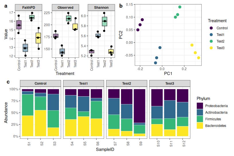
What we are building: reads retained per sample, ASV counts, alpha diversity (Shannon, observed features, Faith’s PD), beta diversity (Bray-Curtis PCoA + PERMANOVA), and stacked taxonomy barplots at phylum, family, and genus level — all combined into a single multi-panel figure.

What you need before starting

This guide assumes you have already completed the QIIME 2 analysis (import → trim → DADA2 → taxonomy → filtering → core metrics). Your working directory should contain files like these:

table-no-contam_240_200.qza
taxonomy_240_200.qza
denoising-stats_240_200.qza
rooted-tree_240_200.qza
core-metrics-results_50000/
my_metadata.txt

File names will vary by project — adapt them throughout.

see_your_Genome

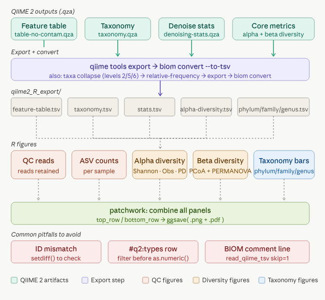
Part 1: Exporting from QIIME 2

QIIME 2 stores everything in .qza and .qzv files, which are essentially zip archives with provenance tracking. Before R can read them, you need to export the underlying data files.

Step 1: Create a clean export directory

Keep all exported files together in one folder. This makes paths in R much simpler.

mkdir -p qiime2_R_export

Step 2: Export the feature table

qiime tools export \
  --input-path table-no-contam_240_200.qza \
  --output-path qiime2_R_export/table

This creates qiime2_R_export/table/feature-table.biom. BIOM is a compressed binary format — R cannot read it directly, so we convert it to TSV:

biom convert \
  -i qiime2_R_export/table/feature-table.biom \
  -o qiime2_R_export/table/feature-table.tsv \
  --to-tsv

Step 3: Export taxonomy

qiime tools export \
  --input-path taxonomy_240_200.qza \
  --output-path qiime2_R_export/taxonomy

This produces taxonomy.tsv — a two-column file with feature IDs and their SILVA taxonomy strings.

Step 4: Export denoising statistics

qiime tools export \
  --input-path denoising-stats_240_200.qza \
  --output-path qiime2_R_export/denoising_stats

This gives you stats.tsv — the per-sample read counts at every DADA2 step (input → filtered → denoised → merged → non-chimeric). This is important for quality checking.

Step 5: Export alpha diversity vectors

qiime tools export \
  --input-path core-metrics-results_50000/shannon_vector.qza \
  --output-path qiime2_R_export/shannon

qiime tools export \
  --input-path core-metrics-results_50000/observed_features_vector.qza \
  --output-path qiime2_R_export/observed_features

qiime tools export \
  --input-path core-metrics-results_50000/faith_pd_vector.qza \
  --output-path qiime2_R_export/faith_pd

Each of these exports a simple two-column TSV: sample ID and diversity value.

Step 6: Export beta diversity outputs

qiime tools export \
  --input-path core-metrics-results_50000/bray_curtis_distance_matrix.qza \
  --output-path qiime2_R_export/bray_distance

qiime tools export \
  --input-path core-metrics-results_50000/bray_curtis_pcoa_results.qza \
  --output-path qiime2_R_export/bray_pcoa

Step 7: Collapse taxonomy and convert to relative abundance

For stacked barplots, you want the feature table aggregated at phylum, family, and genus level. QIIME 2 does this cleanly with taxa collapse.

SILVA taxonomy levels:

Level 2 = Phylum
Level 5 = Family
Level 6 = Genus

# Collapse
qiime taxa collapse \
  --i-table table-no-contam_240_200.qza \
  --i-taxonomy taxonomy_240_200.qza \
  --p-level 2 \
  --o-collapsed-table phylum.qza

qiime taxa collapse \
  --i-table table-no-contam_240_200.qza \
  --i-taxonomy taxonomy_240_200.qza \
  --p-level 5 \
  --o-collapsed-table family.qza

qiime taxa collapse \
  --i-table table-no-contam_240_200.qza \
  --i-taxonomy taxonomy_240_200.qza \
  --p-level 6 \
  --o-collapsed-table genus.qza

# Convert to relative abundance
qiime feature-table relative-frequency --i-table phylum.qza --o-relative-frequency-table phylum_rel.qza
qiime feature-table relative-frequency --i-table family.qza --o-relative-frequency-table family_rel.qza
qiime feature-table relative-frequency --i-table genus.qza  --o-relative-frequency-table genus_rel.qza

# Export
qiime tools export --input-path phylum_rel.qza --output-path qiime2_R_export/phylum
qiime tools export --input-path family_rel.qza --output-path qiime2_R_export/family
qiime tools export --input-path genus_rel.qza  --output-path qiime2_R_export/genus

# Convert BIOM to TSV for each
cd qiime2_R_export
biom convert -i phylum/feature-table.biom -o phylum/feature-table.tsv --to-tsv
biom convert -i family/feature-table.biom -o family/feature-table.tsv --to-tsv
biom convert -i genus/feature-table.biom  -o genus/feature-table.tsv  --to-tsv

Step 8: Copy your metadata

cp my_metadata.txt qiime2_R_export/

What your export folder should look like

qiime2_R_export/
├── table/
│   ├── feature-table.biom
│   └── feature-table.tsv
├── taxonomy/
│   └── taxonomy.tsv
├── denoising_stats/
│   └── stats.tsv
├── shannon/
│   └── alpha-diversity.tsv
├── observed_features/
│   └── alpha-diversity.tsv
├── faith_pd/
│   └── alpha-diversity.tsv
├── bray_distance/
│   └── distance-matrix.tsv
├── bray_pcoa/
│   └── ordination.txt
├── phylum/
│   └── feature-table.tsv
├── family/
│   └── feature-table.tsv
├── genus/
│   └── feature-table.tsv
└── my_metadata.txt

Part 2: Visualization in R

Set your working directory to the export folder first:

setwd("path/to/qiime2_R_export")

Libraries

library(tidyverse)   # data manipulation + ggplot2
library(vegan)       # PERMANOVA (adonis2)
library(biomformat)  # read BIOM files if needed
library(viridis)     # colour palettes
library(patchwork)   # combine multiple plots
library(cowplot)     # draw_label for text panels

A: Read metadata

Your metadata file is the anchor that connects every other file. Every sample ID in every TSV must match the IDs here exactly.

meta <- read.delim("my_metadata.txt", sep = "\t", check.names = FALSE)
colnames(meta)[1] <- "SampleID"

# Set a sensible factor order for treatments
meta$Treatment <- factor(meta$Treatment, levels = c("NC", "NPK", "nOB9"))

B: Denoising statistics — how many reads did DADA2 keep?

denoise <- read.delim("denoising_stats/stats.tsv",
                      sep = "\t", check.names = FALSE, stringsAsFactors = FALSE)

# Clean column names (QIIME2 uses hyphens and spaces)
colnames(denoise) <- gsub("[-  ]", "_", colnames(denoise))
colnames(denoise)[1] <- "SampleID"

# Remove the QIIME2 type annotation row
denoise <- denoise[denoise$SampleID != "#q2:types", ]

# Convert counts to numeric
num_cols <- setdiff(colnames(denoise), "SampleID")
denoise[num_cols] <- lapply(denoise[num_cols], as.numeric)

Why the #q2:types row? QIIME 2 metadata files include a second header row that describes data types (e.g. numeric, categorical). It looks like data but it is metadata about the metadata. Always remove it before any numeric conversion.

reads_plot <- ggplot(denoise, aes(x = SampleID, y = non_chimeric, fill = SampleID)) +
  geom_col() +
  theme_bw() +
  labs(title = "Reads retained after DADA2", x = NULL, y = "Non-chimeric reads") +
  theme(axis.text.x = element_text(angle = 45, hjust = 1), legend.position = "none")

C: ASV counts per sample

library(biomformat)

table_biom <- read_biom("table/feature-table.biom")
asv_mat    <- as.data.frame(as.matrix(biom_data(table_biom)))

asv_per_sample <- colSums(asv_mat)
asv_df         <- data.frame(SampleID = names(asv_per_sample), ASV_count = asv_per_sample)

asv_plot <- ggplot(asv_df, aes(x = SampleID, y = ASV_count, fill = SampleID)) +
  geom_col() +
  theme_bw() +
  labs(title = "Total ASV abundance per sample", x = NULL, y = "Total ASV abundance") +
  theme(axis.text.x = element_text(angle = 45, hjust = 1), legend.position = "none")

D: Alpha diversity — Shannon, observed features, Faith’s PD

shannon <- read.delim("shannon/alpha-diversity.tsv",          sep = "\t")
obs     <- read.delim("observed_features/alpha-diversity.tsv", sep = "\t")
faith   <- read.delim("faith_pd/alpha-diversity.tsv",          sep = "\t")

colnames(shannon) <- c("SampleID", "Shannon")
colnames(obs)     <- c("SampleID", "Observed")
colnames(faith)   <- c("SampleID", "FaithPD")

alpha_df <- meta %>%
  left_join(shannon, by = "SampleID") %>%
  left_join(obs,     by = "SampleID") %>%
  left_join(faith,   by = "SampleID")

Plot all three metrics on one faceted panel:

alpha_long <- alpha_df %>%
  pivot_longer(cols = c(Shannon, Observed, FaithPD),
               names_to = "Metric", values_to = "Value")

alpha_plot <- ggplot(alpha_long, aes(x = Treatment, y = Value, fill = Treatment)) +
  geom_boxplot(alpha = 0.5, outlier.shape = NA) +
  geom_jitter(width = 0.1, size = 2) +
  facet_wrap(~ Metric, scales = "free_y") +
  scale_fill_viridis_d(option = "plasma") +
  theme_bw() +
  labs(title = "Alpha diversity", x = NULL, y = NULL) +
  theme(strip.text = element_text(face = "bold"), legend.position = "none")

Optional: statistical testing

kruskal.test(Shannon ~ Treatment, data = alpha_df)
kruskal.test(Observed ~ Treatment, data = alpha_df)
kruskal.test(FaithPD  ~ Treatment, data = alpha_df)

# Pairwise comparisons
pairwise.wilcox.test(alpha_df$Shannon, alpha_df$Treatment, p.adjust.method = "BH")

What these metrics mean:

Shannon index — accounts for both richness (how many taxa) and evenness (how evenly distributed). Higher = more diverse.
Observed features — simply the count of unique ASVs detected. Sensitive to sampling depth.
Faith’s PD — phylogenetic diversity. Sums the branch lengths of the phylogenetic tree covered by the detected ASVs. Higher = more evolutionary breadth.

E: Beta diversity — Bray-Curtis PCoA + PERMANOVA

Reading the PCoA ordination file requires a small trick: QIIME 2 writes a header with metadata about eigenvalues above the coordinate data. We skip 4 lines to get to the actual coordinates.

pcoa <- read.delim("bray_pcoa/ordination.txt",
                   sep = "\t", skip = 4, check.names = FALSE,
                   row.names = 1)

# Keep only sample rows (not the "Site" or "Species" annotation rows)
coords <- pcoa[!(rownames(pcoa) %in% c("Species", "Site")), 1:2, drop = FALSE]
coords$SampleID <- rownames(coords)
colnames(coords) <- c("PC1", "PC2", "SampleID")

coords$PC1 <- as.numeric(coords$PC1)
coords$PC2 <- as.numeric(coords$PC2)

ord_df <- left_join(coords, meta, by = "SampleID")

PERMANOVA tests whether treatment groups have significantly different community composition:

dist_mat <- read.delim("bray_distance/distance-matrix.tsv",
                       sep = "\t", row.names = 1, check.names = FALSE)
dist_obj <- as.dist(dist_mat)

adon <- adonis2(dist_obj ~ Treatment, data = meta, permutations = 999)
pval <- adon$`Pr(>F)`[1]
r2   <- adon$R2[1]

beta_plot <- ggplot(ord_df, aes(PC1, PC2, color = Treatment)) +
  geom_point(size = 3) +
  stat_ellipse() +
  theme_bw() +
  labs(title = paste0("Bray-Curtis PCoA\nPERMANOVA p=", signif(pval, 3),
                      ", R²=", round(r2, 3)),
       x = "PC1", y = "PC2")

What PERMANOVA R² means: the proportion of community variation explained by the grouping variable. R² = 0.35 means 35% of the variation between samples is associated with treatment.

Pairwise PERMANOVA (which specific treatments differ from each other?):

pairwise_adonis <- function(dist, factors) {
  comb <- combn(unique(factors), 2)
  results <- data.frame()
  for (i in 1:ncol(comb)) {
    group <- comb[, i]
    idx   <- factors %in% group
    sub_dist <- as.dist(as.matrix(dist)[idx, idx])
    sub_meta <- data.frame(Treatment = factors[idx])
    ad <- adonis2(sub_dist ~ Treatment, data = sub_meta)
    results <- rbind(results, data.frame(Group1=group[1], Group2=group[2],
                                         R2=ad$R2[1], p=ad$`Pr(>F)`[1]))
  }
  results$p_adj <- p.adjust(results$p, method = "BH")
  results
}

pairwise_adonis(dist_obj, meta$Treatment)

F: Taxonomy helper functions

Two small functions make all the taxonomy plots reusable.

Helper 1: Read a QIIME 2 TSV

read_qiime_tsv <- function(path) {
  x <- read.delim(path, sep = "\t", header = TRUE,
                  comment.char = "", check.names = FALSE,
                  stringsAsFactors = FALSE, skip = 1)
  colnames(x)[1] <- "Taxon"
  x
}

The skip = 1 is important — BIOM-converted TSVs start with a comment line (# Constructed from biom file) that is not data.

Helper 2: Clean SILVA taxonomy strings

SILVA taxonomy strings look like: d__Bacteria;p__Proteobacteria;c__Gammaproteobacteria;.... The function below pulls out the level you want and strips the prefix.

extract_tax_label <- function(taxon_string, level = c("phylum","family","genus")) {
  level <- match.arg(level)
  sapply(taxon_string, function(x) {
    parts <- trimws(unlist(strsplit(x, ";")))
    val <- switch(level,
                  phylum = parts[2],
                  family = parts[5],
                  genus  = parts[6])
    if (length(val) == 0 || is.na(val) || val == "") return("Unassigned")
    val <- sub("^[a-z]__", "", val)
    if (val %in% c("", "uncultured", "metagenome", "Ambiguous_taxa")) return("Unassigned")
    val
  })
}

Helper 3: Build a long-format taxonomy table

make_long_taxa <- function(path, meta, level = c("phylum","family","genus")) {
  level <- match.arg(level)
  tab   <- read_qiime_tsv(path)
  tab %>%
    pivot_longer(-Taxon, names_to = "SampleID", values_to = "Abundance") %>%
    mutate(Abundance = as.numeric(Abundance),
           Label = extract_tax_label(Taxon, level = level)) %>%
    group_by(SampleID, Label) %>%
    summarise(Abundance = sum(Abundance, na.rm = TRUE), .groups = "drop") %>%
    left_join(meta, by = "SampleID")
}

G: Stacked taxonomy barplots

plot_taxa_stacked <- function(long_df, title_txt, top_n = 15) {

  # Identify top N taxa by total abundance
  top_taxa <- long_df %>%
    group_by(Label) %>%
    summarise(Total = sum(Abundance, na.rm = TRUE), .groups = "drop") %>%
    arrange(desc(Total)) %>%
    slice_head(n = top_n) %>%
    pull(Label)

  # Merge everything else into "Other"
  plot_df <- long_df %>%
    mutate(Label = ifelse(Label %in% top_taxa, Label, "Other")) %>%
    group_by(SampleID, Treatment, Label) %>%
    summarise(Abundance = sum(Abundance, na.rm = TRUE), .groups = "drop")

  # Order fill by overall abundance
  levs <- plot_df %>%
    group_by(Label) %>%
    summarise(Total = sum(Abundance), .groups = "drop") %>%
    arrange(desc(Total)) %>% pull(Label)
  plot_df$Label     <- factor(plot_df$Label, levels = rev(unique(levs)))
  plot_df$SampleID  <- factor(plot_df$SampleID, levels = levels(meta$SampleID))
  plot_df$Treatment <- factor(plot_df$Treatment, levels = levels(meta$Treatment))

  ggplot(plot_df, aes(x = SampleID, y = Abundance, fill = Label)) +
    geom_col(width = 0.9, colour = "white", linewidth = 0.1) +
    scale_fill_viridis_d(option = "turbo") +
    scale_y_continuous(labels = function(x) paste0(round(x * 100), "%")) +
    facet_grid(. ~ Treatment, scales = "free_x", space = "free_x") +
    labs(title = title_txt, x = "Sample", y = "Relative abundance", fill = NULL) +
    theme_bw() +
    theme(axis.text.x = element_text(angle = 90, vjust = 0.5, hjust = 1),
          panel.grid = element_blank(),
          strip.background = element_rect(fill = "white"),
          strip.text = element_text(face = "bold"))
}

# Build the three tables
phylum_long <- make_long_taxa("phylum/feature-table.tsv", meta, "phylum")
family_long <- make_long_taxa("family/feature-table.tsv", meta, "family")
genus_long  <- make_long_taxa("genus/feature-table.tsv",  meta, "genus")

# Build the three plots
phylum_plot <- plot_taxa_stacked(phylum_long, "Phylum-level relative abundance", top_n = 12)
family_plot <- plot_taxa_stacked(family_long, "Family-level relative abundance",  top_n = 20)
genus_plot  <- plot_taxa_stacked(genus_long,  "Genus-level relative abundance",   top_n = 20)

H: Text summary panel

This creates a plain-text summary card that works well in the top-left corner of a multi-panel figure.

total_input   <- sum(denoise$input,        na.rm = TRUE)
total_nonchim <- sum(denoise$non_chimeric, na.rm = TRUE)
avg_nonchim   <- mean(denoise$non_chimeric, na.rm = TRUE)

summary_text <- ggdraw() +
  draw_label(
    paste0(
      "16S Amplicon Summary\n\n",
      "Total input reads:  ", format(total_input,   big.mark = ","), "\n",
      "Retained reads:     ", format(total_nonchim, big.mark = ","), "\n",
      "Average per sample: ", round(avg_nonchim, 0), "\n",
      "Samples:            ", nrow(meta), "\n",
      "ASVs detected:      ", nrow(asv_mat)
    ),
    x = 0.05, hjust = 0, vjust = 1, size = 12
  )

I: Combine everything into one figure

top_row    <- summary_text | reads_plot | asv_plot | alpha_plot | beta_plot
bottom_row <- phylum_plot  | family_plot | genus_plot

final_plot <- top_row / bottom_row + plot_layout(heights = c(1, 1.1))

ggsave("reference_style_figure.png", final_plot, width = 22, height = 12, dpi = 300)
ggsave("reference_style_figure.pdf", final_plot, width = 22, height = 12)

Part 3: Bonus — taxon-focused plots

Sometimes you want to zoom into a specific group. In the Bacillus inoculant study, the question was whether different treatments altered the abundance of rhizobia — the nitrogen-fixing bacteria.

Rhizobia genera plot

rhizobia_genera <- c(
  "Rhizobium", "Bradyrhizobium", "Mesorhizobium", "Ensifer",
  "Sinorhizobium", "Azorhizobium", "Allorhizobium", "Neorhizobium",
  "Pararhizobium", "Shinella", "Devosia", "Microvirga"
)

# Keep only rhizobia rows
rhizobia_only <- genus_long %>%
  filter(Label %in% rhizobia_genera) %>%
  group_by(SampleID, Treatment, Label) %>%
  summarise(Abundance = sum(Abundance, na.rm = TRUE), .groups = "drop")

rhizobia_only$SampleID  <- factor(rhizobia_only$SampleID,  levels = levels(meta$SampleID))
rhizobia_only$Treatment <- factor(rhizobia_only$Treatment, levels = levels(meta$Treatment))

# Custom colours so "Other" is always grey
taxa_no_other <- unique(rhizobia_only$Label)
cols <- setNames(viridis::viridis(length(taxa_no_other), option = "turbo"), taxa_no_other)

rhizobia_plot <- ggplot(rhizobia_only,
                        aes(x = SampleID, y = Abundance, fill = Label)) +
  geom_col(width = 0.9, colour = "white", linewidth = 0.1) +
  scale_fill_manual(values = cols) +
  scale_y_continuous(labels = scales::percent_format(accuracy = 0.01)) +
  facet_grid(. ~ Treatment, scales = "free_x", space = "free_x") +
  labs(title = "Rhizobia-related genera (zoomed)", x = "Sample",
       y = "Relative abundance", fill = NULL) +
  theme_bw() +
  theme(axis.text.x = element_text(angle = 90, vjust = 0.5, hjust = 1),
        panel.grid = element_blank(),
        strip.text = element_text(face = "bold"))

Total rhizobia abundance per treatment (boxplot)

rhizobia_total <- genus_long %>%
  mutate(is_rhizobia = Label %in% rhizobia_genera) %>%
  group_by(SampleID, Treatment) %>%
  summarise(Rhizobia = sum(Abundance[is_rhizobia]), .groups = "drop")

ggplot(rhizobia_total, aes(Treatment, Rhizobia, fill = Treatment)) +
  geom_boxplot(alpha = 0.5) +
  geom_jitter(width = 0.1, size = 2) +
  scale_y_continuous(labels = scales::percent) +
  theme_bw() +
  labs(title = "Total rhizobia abundance by treatment")

Common beginner mistakes

Metadata IDs do not match sample IDs in the table

This is the most common silent failure. Your left_join(coords, meta, by = "SampleID") will produce rows full of NA if IDs differ even by a trailing space or capital letter. Always run:

setdiff(colnames(asv_mat), meta$SampleID)  # in table but not in metadata
setdiff(meta$SampleID, colnames(asv_mat))  # in metadata but not in table

Both should return character(0). If not, fix the metadata file or use trimws() on your IDs.

The #q2:types row breaks numeric conversion

QIIME 2 metadata files include a second header row describing types. It looks like a data row but contains strings like "numeric" or "categorical". Always filter it out before calling as.numeric().

denoise <- denoise[denoise$SampleID != "#q2:types", ]

BIOM-to-TSV conversion produces a comment line

The first line of a BIOM-converted TSV is # Constructed from biom file. The read_qiime_tsv() helper above uses skip = 1 to ignore it. If you use read.delim() directly without skipping, R will read this comment as the header — and all your column names will be wrong.

PCoA ordination file has non-sample rows

The QIIME 2 ordination file has rows called "Species" and "Site" below the coordinate data. Always filter them out:

coords <- pcoa[!(rownames(pcoa) %in% c("Species", "Site")), ]

Stacked barplots with raw counts instead of relative abundance

Make sure you used phylum_rel.qza (after qiime feature-table relative-frequency) and not the raw phylum.qza. Raw counts make barplots uninterpretable when samples have different total read depths.

Summary: what does each output file contain?

File	What is in it	R use
`table/feature-table.tsv`	ASVs × samples raw counts	Count checks, richness
`taxonomy/taxonomy.tsv`	Feature ID → SILVA taxonomy	Taxonomy parsing
`denoising_stats/stats.tsv`	Per-sample DADA2 read retention	QC plot
`shannon/alpha-diversity.tsv`	Shannon index per sample	Alpha plot
`observed_features/alpha-diversity.tsv`	ASV count per sample (rarefied)	Alpha plot
`faith_pd/alpha-diversity.tsv`	Phylogenetic diversity per sample	Alpha plot
`bray_distance/distance-matrix.tsv`	Pairwise Bray-Curtis distances	PERMANOVA
`bray_pcoa/ordination.txt`	PCoA coordinates	Beta diversity plot
`phylum/feature-table.tsv`	Relative abundance collapsed to phylum	Stacked barplot
`family/feature-table.tsv`	Relative abundance collapsed to family	Stacked barplot
`genus/feature-table.tsv`	Relative abundance collapsed to genus	Stacked barplot

Statistics

You can also do simple statistics on the diversity analysis like below.

############################################################
# Simple stats for alpha and beta diversity
############################################################

library(tidyverse)
library(vegan)

# ==========================
# 1. Load data
# ==========================
# Replace with your paths
meta <- read.delim("my_metadata.txt", sep = "\t")
shannon <- read.delim("shannon/alpha-diversity.tsv", sep = "\t")
observed <- read.delim("observed_features/alpha-diversity.tsv", sep = "\t")
faith <- read.delim("faith_pd/alpha-diversity.tsv", sep = "\t")

colnames(shannon) <- c("SampleID", "Shannon")
colnames(observed) <- c("SampleID", "Observed")
colnames(faith) <- c("SampleID", "FaithPD")

# Merge
alpha_df <- meta %>%
  left_join(shannon, by = "SampleID") %>%
  left_join(observed, by = "SampleID") %>%
  left_join(faith, by = "SampleID")

alpha_df$Treatment <- factor(alpha_df$Treatment)

# ==========================
# 2. Alpha diversity stats
# ==========================

# ---- Kruskal-Wallis (global)
kw_shannon <- kruskal.test(Shannon ~ Treatment, data = alpha_df)
kw_observed <- kruskal.test(Observed ~ Treatment, data = alpha_df)
kw_faith <- kruskal.test(FaithPD ~ Treatment, data = alpha_df)

kw_shannon
kw_observed
kw_faith

# ---- Pairwise Wilcoxon
pw_shannon <- pairwise.wilcox.test(alpha_df$Shannon, alpha_df$Treatment, p.adjust.method = "BH")
pw_observed <- pairwise.wilcox.test(alpha_df$Observed, alpha_df$Treatment, p.adjust.method = "BH")
pw_faith <- pairwise.wilcox.test(alpha_df$FaithPD, alpha_df$Treatment, p.adjust.method = "BH")

pw_shannon
pw_observed
pw_faith

# ==========================
# 3. Beta diversity stats
# ==========================

# Load Bray-Curtis distance matrix
dist_mat <- read.delim("bray_distance/distance-matrix.tsv",
                       sep = "\t", row.names = 1)

dist_obj <- as.dist(dist_mat)

# ---- PERMANOVA
adon <- adonis2(dist_obj ~ Treatment, data = meta, permutations = 999)
adon

# Extract values
pval <- adon$`Pr(>F)`[1]
r2 <- adon$R2[1]

cat("PERMANOVA: R2 =", r2, "p =", pval, "\n")

# ==========================
# 4. Pairwise PERMANOVA
# ==========================

pairwise_adonis <- function(dist, factors) {
  comb <- combn(unique(factors), 2)
  results <- data.frame()

  for(i in 1:ncol(comb)){
    group <- comb[,i]
    idx <- factors %in% group

    sub_dist <- as.dist(as.matrix(dist)[idx, idx])
    sub_meta <- data.frame(Treatment = factors[idx])

    ad <- adonis2(sub_dist ~ Treatment, data = sub_meta)

    results <- rbind(results, data.frame(
      Group1 = group[1],
      Group2 = group[2],
      R2 = ad$R2[1],
      p = ad$`Pr(>F)`[1]
    ))
  }

  results$p_adj <- p.adjust(results$p, method = "BH")
  results
}

pairwise_results <- pairwise_adonis(dist_obj, meta$Treatment)
pairwise_results

# ==========================
# 5. Dispersion test (IMPORTANT)
# ==========================

disp <- betadisper(dist_obj, meta$Treatment)
anova_disp <- anova(disp)

anova_disp

# ==========================
# 6. Save summary tables
# ==========================

alpha_summary <- data.frame(
  Metric = c("Shannon", "Observed", "FaithPD"),
  p_value = c(kw_shannon$p.value, kw_observed$p.value, kw_faith$p.value)
)

write.csv(alpha_summary, "alpha_stats.csv", row.names = FALSE)
write.csv(pairwise_results, "pairwise_permanova.csv", row.names = FALSE)

Repository

For detailed R scripts and other files see this Repository

This workflow covers the Bacillus inoculant soil microbiome project (16S V4 amplicons, 9 samples across NC/NPK/nOB9 treatments, SILVA 138, DADA2 pseudo-pooling, sampling depth 50,000 reads). The same pipeline applies to any QIIME 2 amplicon dataset — adapt file names and taxonomy level labels to your study.

Tags: QIIME2 16S amplicon R ggplot2 alpha-diversity beta-diversity taxonomy DADA2 PERMANOVA microbiome beginner

see_your_plot