Day 4 — Reads Meet Reference: The Mapping & Quantification Pipeline
*🧬 Day 68 of Daily Bioinformatics from Jojy’s Desk🧬
This is where the analysis becomes concrete.
Three days of preparation — quality control, rRNA removal, paired-end repair, reference construction — have led here. Your reads are clean. Your reference is indexed. Your read pairs are synchronized. Now you are going to find out which genes were being expressed in your estuarine community, and how many reads support each one.
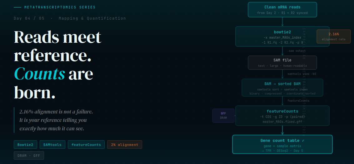
The pipeline has four stages: mapping (Bowtie2), format conversion (SAM → BAM), sorting and indexing (SAMtools), and quantification (featureCounts). We will walk through every command, show you the real output from our dataset, and — critically — explain what the numbers mean when they look alarming.
Before you start: a quick checklist
Before running any mapping command, verify these three things. Every mapping failure I have seen in the analysis traces back to one of them:
# 1. Are your mRNA reads where you expect them?
ls mRNA_reads/
# Should show: CP_Spr15G08_mRNA_fwd.fq  CP_Spr15G08_mRNA_rev.fq
# (and the same pattern for all other samples)

# 2. Are R1 and R2 synchronized?
echo "R1: $(cat mRNA_reads/CP_Spr15G08_mRNA_fwd.fq | wc -l | awk '{print $1/4}')"
echo "R2: $(cat mRNA_reads/CP_Spr15G08_mRNA_rev.fq | wc -l | awk '{print $1/4}')"
# These two numbers MUST be identical — see Day 2 repair scripts if not

# 3. Does your Bowtie2 index exist?
ls MAGS/bowtie_index/
# Should show six files: master_MAGs_index.1.bt2 through master_MAGs_index.rev.2.bt2
# If missing: run Day 3 script 01_build_mag_index.slurm first
If all three pass, you are ready. If any fail, stop and fix them first — do not run Bowtie2 with broken input.
Prebuilt Bowtie Index
A pre-built Bowtie2 index generated from 3–4 MAGs is now available in the Day 1 repository (bowtie_index. This allows you to skip the indexing step and directly run the mapping workflow.
Stage 1 — Bowtie2: mapping reads to the reference
Bowtie2 takes your clean RNA reads and searches the reference index for matching sequences. For each read, it either finds a location in the reference (a mapping) or it doesn’t. The result is a SAM file recording every read, where it mapped (or that it didn’t), and how confidently.
module load bowtie2/2.5.4
If you want to install it refer : https://github.com/benlangmead/bowtie2
bowtie2 \
  -x /project/bcampb7/camplab/MICRO_8130_2026/metatranscriptome/MAGS/bowtie_index/master_MAGs_index \
  -1 mRNA_reads/CP_Spr15G08_mRNA_fwd.fq \
  -2 mRNA_reads/CP_Spr15G08_mRNA_rev.fq \
  -p 8 \
  --no-unal \
  --very-sensitive \
  -S CP_Spr15G08.sam \
  2> logs/CP_Spr15G08_bowtie2.log
What each flag means — explained for beginners:
| Flag | What it does | Why it matters |
|---|---|---|
-x | Path to the index prefix | Points Bowtie2 to the six .bt2 files you built on Day 3. Leave off the .bt2 extension — Bowtie2 finds them automatically |
-1 / -2 | R1 and R2 read files | Always provide both. Your reads are paired — Bowtie2 needs both mates to attempt concordant mapping |
-p 8 | Use 8 CPU threads | Match this to your --cpus-per-task SLURM allocation. More threads = faster, not more reads |
--no-unal | Do not write unmapped reads to SAM | Critical for low-alignment-rate datasets. Without this flag, 98% of your reads (unmapped) inflate the SAM file to many GB for no benefit |
--very-sensitive | More thorough alignment search | Environmental reads are often divergent from your reference. This flag tells Bowtie2 to try harder before giving up on a read |
-S | Output SAM file | The alignment result. One line per read |
2> | Redirect stderr to a log file | Bowtie2 prints its alignment statistics to stderr, not stdout. Capturing it means you can check the stats later without re-running |
Reading the alignment statistics: what the numbers mean
When Bowtie2 finishes, check the log file you captured:
cat logs/CP_Spr15G08_bowtie2.log
Here is the real output from our estuarine dataset:
3647405 reads; of these:
  3647405 (100.00%) were paired; of these:
    3647405 (100.00%) aligned concordantly 0 times
    0 (0.00%) aligned concordantly exactly 1 time
    0 (0.00%) aligned concordantly >1 times
    ----
    3647405 pairs aligned concordantly 0 times; of these:
      1747 (0.05%) aligned discordantly 1 time
    ----
    3645658 pairs aligned 0 times concordantly or discordantly; of these:
      7291316 mates make up the pairs; of these:
        7137598 (97.89%) aligned 0 times
        152441 (2.09%) aligned exactly 1 time
        1277 (0.02%) aligned >1 times
2.16% overall alignment rate
This output has a specific structure. Let’s decode it line by line.
“aligned concordantly 0 times: 100%”
This is the line that makes beginners panic. It means zero read pairs mapped in the expected orientation — both mates on the same contig, pointing inward, within the expected insert size. In a genome resequencing experiment, 100% concordant failure is catastrophic. Here, it is expected.
Our four MAGs contain 1,274 contigs, each typically a few thousand basepairs long. For a pair to map concordantly, both mates need to land on the same contig. With such short, fragmented reference contigs and only four organisms represented, the chance of both mates from any given pair both happening to hit our reference is very small. This is a geometry problem, not a quality problem.
“152,441 (2.09%) aligned exactly 1 time”
This is your actual signal. These are individual mates that found a unique, unambiguous match in your reference. A uniquely mapped read is the gold standard — it came from exactly one place in the reference, with high confidence. 152,441 of these is not a lot, but it is real biological signal from the organisms in your four MAGs.
“2.16% overall alignment rate”
Your headline number. 157,212 reads mapped out of 7.3 million. The rest — from the hundreds of estuarine taxa not in your four MAGs — found nothing to match against and were discarded by --no-unal.
Repeat this until it feels true: 2% is not a failure. It means your four MAGs captured approximately 2% of the expressed community. The 98% that didn’t map are not lost data — they are a reminder that your reference is a window, not the whole room. As you add more MAGs or switch to a reference database (Day 3), this number will climb.
Stage 2 — SAMtools: SAM to sorted BAM
The SAM file Bowtie2 produces is a plain text file. Every mapped read occupies one line. For a dataset with 157,000 mapped reads, this is manageable. For a dataset with millions of reads at high alignment rates, SAM files become enormous — tens or hundreds of GB — and are slow to work with.
BAM is the binary (compressed) version of SAM. Same information, a fraction of the file size, and orders of magnitude faster for every downstream tool. We always convert immediately.
Sorted BAM organizes alignments by their position along each reference contig. featureCounts requires this. So does IGV if you want to visualize your mappings. Always sort.
module load samtools

# Step 1: Convert SAM to BAM
samtools view \
  -bS \
  -@ 8 \
  CP_Spr15G08.sam > CP_Spr15G08.bam

# Step 2: Sort by genomic coordinate
samtools sort \
  -@ 8 \
  -m 4G \
  CP_Spr15G08.bam \
  -o CP_Spr15G08_sorted.bam

# Step 3: Index the sorted BAM
# (creates CP_Spr15G08_sorted.bam.bai)
samtools index CP_Spr15G08_sorted.bam

# Step 4: Remove the unsorted BAM and SAM to save disk space
rm CP_Spr15G08.bam CP_Spr15G08.sam
Flag explanation:
-
samtools view -bS—-b= output BAM format;-S= input is SAM format -
-@ 8— use 8 threads (works for bothviewandsort) -
-m 4G— allow each thread up to 4 GB RAM during sorting (prevents disk spill on large files) -
samtools index— creates a.baiindex file next to the BAM; required for featureCounts and visualization tools
Disk space tip: Delete your SAM files after converting to BAM. A SAM file for 157,000 mapped reads with
--no-unalis small, but if you run without--no-unal, your SAM files can be 10–50× larger than the BAM. Always clean up.
Stage 3 — SAMtools flagstat: understanding your alignments
Before running featureCounts, always run flagstat. It gives you a concise diagnostic of what is actually in your BAM file:
samtools flagstat CP_Spr15G08_sorted.bam
Real output from our dataset:
7294810 + 0 in total (QC-passed reads + QC-failed reads)
7294810 + 0 primary
0 + 0 secondary
0 + 0 supplementary
0 + 0 duplicates
157212 + 0 mapped (2.16% : N/A)
157212 + 0 primary mapped (2.16% : N/A)
7294810 + 0 paired in sequencing
3647405 + 0 read1
3647405 + 0 read2
0 + 0 properly paired (0.00% : N/A)
3566 + 0 with itself and mate mapped
153646 + 0 singletons (2.11% : N/A)
3496 + 0 with mate mapped to a different chr
Reading this output — beginner guide:
| Line | What it means | Our value |
|---|---|---|
in total | Total reads entering SAM/BAM | 7,294,810 (all reads, mapped + unmapped if --no-unal was not used) |
mapped | Reads that aligned to the reference | 157,212 (2.16%) |
properly paired | Both mates mapped to same contig, correct orientation | 0 — expected with fragmented MAG contigs |
with itself and mate mapped | Both mates mapped, but not necessarily same contig | 3,566 — these are real pairs |
singletons | One mate mapped, the other didn’t | 153,646 — one mate hit a MAG gene, other hit nothing |
Why is “properly paired” zero? This confuses almost every beginner. “Properly paired” requires both mates to map to the same contig within the expected insert size (~200–800 bp). Our MAG contigs are short and fragmented. Even when both mates of a pair come from the same organism, they often land on different contigs of that MAG — giving 0% properly paired even when the mapping is biologically valid. This is a reference fragmentation effect, not a data problem.
What about the 153,646 singletons? These are reads where one mate matched a gene in your MAGs and the other mate did not. The mate that mapped is still a valid biological signal — it came from a real gene. featureCounts can handle these with the right flags.
Stage 4 — featureCounts: from alignments to gene counts
featureCounts (from the Subread package) is the counting engine. It reads your sorted BAM and your GFF annotation file, then asks for each read: which annotated gene does this overlap? The result is a count table — one row per gene, one column per sample.
What is a GFF file? A GFF (General Feature Format) file is a text table describing the location of every annotated gene on your reference. Each row describes one feature: which contig it is on, where it starts and ends, which strand it is on, and what its ID is. We use a GFF generated by DRAM annotation of our four MAGs.
module load subread

featureCounts \
  -T 8 \
  -p \
  -B \
  -C \
  -t CDS \
  -g ID \
  -a MAGS/master_MAGs.fixed.gff \
  -o counts/gene_counts_CP_Spr15G08.txt \
  bam/CP_Spr15G08_sorted.bam
Every flag explained:
| Flag | What it does |
|---|---|
-T 8 | Use 8 threads |
-p | Paired-end mode — counts fragments (read pairs), not individual reads. Required for paired data |
-B | Only count reads where both mates map. Remove this if you also want to count singletons |
-C | Do not count chimeric fragments (mates mapping to different chromosomes/contigs). Removes likely noise |
-t CDS | Count reads overlapping CDS (coding sequence) features in the GFF. Use gene if your GFF does not have CDS annotations |
-g ID | Use the ID attribute from the GFF as the gene identifier in the output table |
-a | Your GFF annotation file |
-o | Output count table file |
GFF troubleshooting — the most common featureCounts error: featureCounts fails silently (all zeros) when the sequence IDs in your BAM do not match the sequence IDs in your GFF. This happens when your MAG FASTA headers and your GFF contig names were generated independently. Check with:
grep "^>" MAGS/master_mags.fa | head -5and compare to the first column of your GFF. If they differ, you need to fix the GFF — this is why we usemaster_MAGs.fixed.gff(pre-cleaned for this series).
Running all samples: the batch approach
For a single sample the above commands are fine to run interactively. For three samples — or thirty — you want a single featureCounts call across all BAM files simultaneously. featureCounts produces a single count matrix when given multiple BAM files, which is exactly what you need for downstream analysis:
# After mapping and sorting all three samples:
featureCounts \
  -T 8 \
  -p \
  -B \
  -C \
  -t CDS \
  -g ID \
  -a MAGS/master_MAGs.fixed.gff \
  -o counts/all_samples_counts.txt \
  bam/CP_Spr15G08_sorted.bam \
  bam/CP_Spr15L08_sorted.bam \
  bam/CP_Spr31G08_sorted.bam
The output file all_samples_counts.txt has this structure:
Geneid    Chr    Start    End    Strand    Length    CP_Spr15G08    CP_Spr15L08    CP_Spr31G08
gene_001  contig1  100  900  +  800  0  0  2
gene_002  contig1  950  1800  -  850  4  1  0
gene_003  contig2  200  1100  +  900  0  3  0
...
Most genes will have zero counts — expected, given our 2% alignment rate. A small number of genes will have non-zero counts. Those non-zero counts are your actual signal: real expression from the organisms in your four MAGs. This is the table you carry into Day 5.
Understanding your count table: zeros are not failure
When you open the count table and see hundreds of zeros, resist the instinct to panic. Let’s do the math:
- Our four MAGs have ~1,274 annotated genes (after DRAM annotation)
- 157,212 reads mapped across all genes
- Average reads per gene: ~123
But expression is not uniform. Highly expressed genes (ribosomes, transporters, central metabolism) will absorb most of the reads. Many genes will genuinely have zero expression — either the gene was not active at the time of sampling, or the reads that should have mapped to it were among the 98% from taxa outside our reference.
This zero-inflation is expected in metatranscriptomics, especially with a small reference. It does not mean featureCounts failed. It means your reference is small and your community is large.
What you are looking for: genes with consistent non-zero counts across your samples, or genes with differential counts between conditions (PA vs FL). Even at 2% alignment, if your four MAGs include organisms that are genuinely active in your system, you will see signal.
What’s next
You now have a count table. It is a matrix of integers. By itself, it tells you almost nothing biologically — raw counts are not comparable between samples (different sequencing depths), not normalized for gene length, and not corrected for compositional differences between communities.
Day 5 transforms that matrix into biological insight: TPM normalization, DESeq2 differential expression, DNA:RNA ratios, and ecological interpretation of who is metabolically active in the PA and FL estuarine communities.
Day 5: From Counts to Biology — Normalization, DESeq2, and Ecological Interpretation
📦 All code, SLURM scripts, and toy datasets used in this series are available in the companion repository 📦 Github repository
Questions about this workflow? Drop a comment below. The complete R script and SLURM submission scripts are available in the companion GitHub repository.