Day 3 — The Reference Problem: Your Database Defines Your Biology
The Reference Problem: Your Database Defines Your Biology
🧬 Day 67 of Daily Bioinformatics from Jojy’s Desk🧬
After quality control, your RNA reads are clean, trimmed, rRNA-free, and perfectly synchronized. You are ready to map.
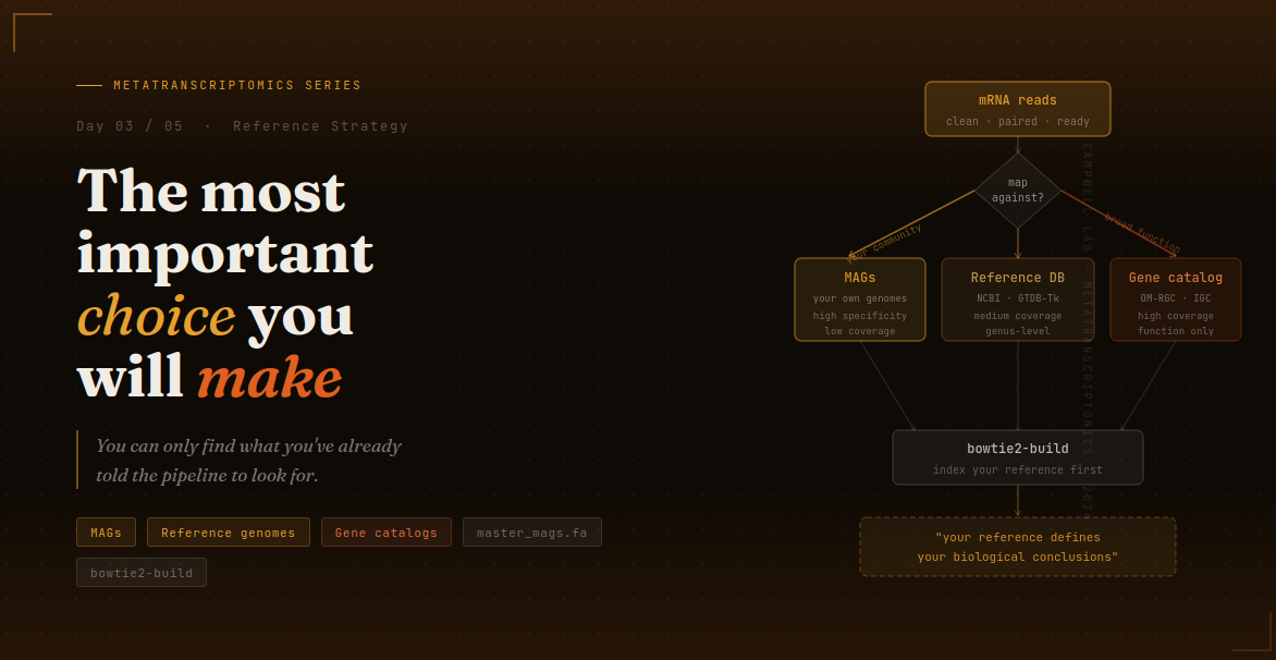
But map to what?
This question — deceptively simple on the surface — is the most consequential decision in your entire metatranscriptomics workflow. Get it wrong and your results will be technically correct but biologically misleading. You will not get an error message. The pipeline will finish. The count table will be generated. And you will draw conclusions that don’t reflect what actually happened in your sample.
Let’s make sure you understand this choice before you make it.
The core concept: you can only find what you look for
Imagine you lose your keys. You search your living room, your kitchen, your bedroom. You don’t find them. What does that tell you?
It tells you your keys are not in those three rooms. It tells you nothing about whether they’re in the garage, the car, or your coat pocket — because you never looked there.
Mapping works the same way. When a read fails to map, it doesn’t mean nothing was expressed. It means the expressed gene is not in your reference. You simply never looked for it.
In a complex environmental sample like an estuarine sediment — where a single gram of sediment can contain thousands of microbial species, most of them never cultured and never sequenced — any reference you build is a small window into a vast room. Your job is to understand exactly how big that window is, and to be honest about what you can and cannot see through it.
The rule: You can only detect what’s in your reference. Everything outside the window is invisible — not absent, just invisible.
What is a reference, exactly?
A reference is a collection of DNA sequences that you believe represent the organisms or genes in your sample. You build an index from those sequences (using bowtie2-build), and then the mapper searches that index for matches to your reads.
Every reference has two properties that matter:
- Coverage — how much of the total community diversity does it represent? A reference with four MAGs covers maybe 2% of an estuarine community. A database with 50,000 reference genomes covers much more.
- Specificity — how closely do the reference sequences match the actual organisms in your sample? Genomes assembled directly from your sample are highly specific. Database genomes from culture collections may be generic representatives that differ meaningfully from your environmental strains.
Coverage and specificity usually trade off against each other. The three reference strategies below sit at different points on this tradeoff.
Strategy 1 — MAGs: high specificity, low coverage
What is a MAG?
A Metagenome-Assembled Genome (MAG) is a draft genome assembled from environmental DNA. You take a paired metagenome from the same samples, assemble the DNA reads into contigs, and then computationally group (bin) those contigs by their coverage patterns and nucleotide composition — hoping that contigs from the same organism cluster together. Each bin is a draft genome of one (or a few) organisms from your community.
MAGs are imperfect — they are partial (a typical high-quality MAG is 70–95% complete), sometimes contaminated with sequences from other organisms, and never perfectly phased. But they are built from your community, which makes them maximally specific to what actually lives in your sample.
Why we use MAGs in this series:
Our four MAGs — MAG1.fasta through MAG4.fasta — were assembled and binned from the same PA and FL estuarine metagenomes we are transcribing. When a read maps to one of these MAGs, we are confident it came from an organism actually present in our system, not a distant relative from a database.
Building the master reference:
The first step is simple: concatenate all your MAGs into a single FASTA file. Bowtie2 maps against one index, so all your reference sequences need to be in one file.
cd /project/bcampb7/camplab/MICRO_8130_2026/metatranscriptome/MAGS

# Concatenate all MAGs
cat MAG1.fasta MAG2.fasta MAG3.fasta MAG4.fasta > master_mags.fa

# Verify: how many contigs do we have?
grep ">" master_mags.fa | wc -l
# Expected: 1274 contigs across 4 MAGs
The honest limitation:
Four MAGs representing 1,274 contigs is a tiny fraction of estuarine community diversity. When we map a whole-community metatranscriptome against this reference on Day 4, we will get approximately 2% overall alignment. That means 98% of the reads — from the hundreds of taxa not represented in our MAGs — will quietly disappear. This is expected. It is not a failure. But you must know it is happening.
A beginner tip: The number of contigs in your reference is a rough proxy for how much of the community you can see. 1,274 contigs across 4 MAGs is a small window. A full GTDB-Tk reference database has millions of contigs — a much bigger window, but with lower specificity.
Strategy 2 — Reference genome databases: medium coverage, medium specificity
Instead of assembling your own genomes, you can map against a curated collection of reference genomes. The most commonly used databases are:
- NCBI RefSeq — the broadest collection; millions of sequences but very uneven coverage across lineages
- GTDB-Tk representative genomes — a phylogenetically curated, non-redundant set of bacterial and archaeal genomes; better for environmental microbiomes than RefSeq
- Environment-specific databases — for example, the TARA Oceans MAG catalog for marine systems, or sediment-specific MAG collections from published studies
When to use this approach:
Use reference databases when you want broader taxonomic coverage than your own MAGs provide, especially for well-characterized lineages like Proteobacteria, Firmicutes, or Actinobacteria. If you’re studying a system where good reference genomes exist (e.g. marine surface water, human gut), a database reference can dramatically improve your alignment rate.
The tradeoff:
A database genome for Sulfurimonas autotrophica might share 90–95% average nucleotide identity (ANI) with your estuarine Sulfurimonas strain. That’s close enough for genus-level expression analysis but may miss strain-specific genes — precisely the genes that might be most ecologically interesting. You are measuring the expression of a cousin, not the actual organism.
Building a database reference:
The workflow is identical to MAGs — concatenate, then build a Bowtie2 index. The difference is file size: a GTDB-Tk representative set can be 50–150 GB, which requires more memory and time to index.
# Example: download and prepare GTDB-Tk representative genomes
# (see SLURM script for full download workflow)

# After download and concatenation:
bowtie2-build \
  --threads 16 \
  --large-index \
  gtdb_representatives.fa \
  gtdb_index

# --large-index is required for references >4 GB
Strategy 3 — Gene catalogs: high coverage, function-focused
Gene catalogs take a completely different approach. Instead of mapping to genomes, you map to a non-redundant collection of predicted protein-coding genes. Each entry in the catalog is a gene (typically 100–1000 bp), clustered at 95% nucleotide identity across many metagenomes.
Major gene catalogs:
- Ocean Microbial Reference Gene Catalog (OM-RGC) — ~46 million non-redundant genes from the TARA Oceans project; excellent for marine systems
- Integrated Gene Catalog (IGC) — built from human gut metagenomes; not appropriate for environmental samples
- Soil Reference Gene Catalog — for soil systems
- Custom catalogs — you can build your own from a set of assembled metagenomes using CD-HIT or MMseqs2
Why use a gene catalog?
Gene catalogs give you the broadest functional coverage. Millions of genes from hundreds of studies means you capture expressed diversity that no individual reference genome set can match. When your question is “what metabolic functions are active in this community?” — not “which specific organism is doing it?” — a gene catalog is the most powerful choice.
The key limitation:
When a read maps to a gene catalog entry, you know the function that was expressed. You do not automatically know the taxonomy of the organism that expressed it, unless you have carefully tracked the provenance of each gene back to its source genome. For ecological questions that depend on linking function to organism identity (like our hydrocarbon degradation work), this is a meaningful limitation.
# Map against a gene catalog (same Bowtie2 workflow, different reference)
bowtie2-build \
  --threads 16 \
  OM-RGC_v2.fa \
  omrgc_index

bowtie2 \
  -x omrgc_index \
  -1 CP_Spr15G08_R1.mRNA.fq \
  -2 CP_Spr15G08_R2.mRNA.fq \
  -p 16 \
  --no-unal \
  -S CP_Spr15G08_omrgc.sam
The --no-unal flag suppresses unmapped reads in the SAM output — essential for gene catalogs where most reads won’t map, and your output files would otherwise be enormous.
Comparing the three strategies
| MAGs | Reference genomes | Gene catalogs | |
|---|---|---|---|
| Coverage | Low (your genomes only) | Medium (known taxa) | High (millions of genes) |
| Specificity | Very high (your community) | Medium (genus level) | Low–medium (function only) |
| Taxonomy | Organism-resolved | Genus-resolved | Poor without extra steps |
| File size | Small (MB) | Large (GB–TB) | Medium–large (GB) |
| Best for | Focused taxa · paired metagenome | Broad surveys · known lineages | Functional profiling · novel environments |
| Our series | ✓ Used here | Discussed as alternative | Discussed as alternative |
The practical recommendation: Do not pick one and ignore the others. The best analyses use MAG-based mapping for high-confidence, organism-resolved expression of your taxa of interest, then complement with a database or gene catalog reference to characterize what your MAGs missed. Think of them as layers, not alternatives.
Our pipeline: building the master_mags.fa index
For this series, we work with four MAGs. Here is the complete workflow from concatenation to index, with verification steps at each stage.
# ── Step 1: navigate to MAG directory ────────────────────────
cd /project/bcampb7/camplab/MICRO_8130_2026/metatranscriptome/MAGS

# ── Step 2: check your MAG files ─────────────────────────────
ls *.fasta
# MAG1.fasta  MAG2.fasta  MAG3.fasta  MAG4.fasta

# How many contigs per MAG?
for f in *.fasta; do
  echo "$f: $(grep -c '>' $f) contigs"
done

# ── Step 3: concatenate into master reference ─────────────────
cat MAG1.fasta MAG2.fasta MAG3.fasta MAG4.fasta > master_mags.fa

# Verify total contig count
grep ">" master_mags.fa | wc -l
# 1274

# ── Step 4: load Bowtie2 and build the index ─────────────────
module load bowtie2/2.5.4

mkdir -p bowtie_index

bowtie2-build \
  master_mags.fa \
  bowtie_index/master_MAGs_index

# ── Step 5: confirm index files were created ──────────────────
ls bowtie_index/
# master_MAGs_index.1.bt2
# master_MAGs_index.2.bt2
# master_MAGs_index.3.bt2
# master_MAGs_index.4.bt2
# master_MAGs_index.rev.1.bt2
# master_MAGs_index.rev.2.bt2
# Six files = successful index build
What are the .bt2 files?
Bowtie2 breaks the index into six files that together encode an FM-index — a compressed data structure that allows rapid substring search across millions of base pairs. You never open these files directly. You point Bowtie2 at them using the prefix (master_MAGs_index), and it handles the rest. You only need to build the index once — reuse it for all samples.
How long does indexing take?
For our four MAGs (~1,274 contigs, a few MB of sequence), indexing finishes in under a minute. For a GTDB-Tk representative database (50 GB+), expect 2–4 hours and 200+ GB of RAM with --large-index.
Understanding what 2% alignment will mean tomorrow
We want to prepare you for what you will see on Day 4 so it does not feel like a failure.
Our master reference has 1,274 contigs from 4 organisms. Our metatranscriptome is a snapshot of hundreds of organisms, all simultaneously expressing thousands of genes. When Bowtie2 searches our small index for matches, the vast majority of reads — from organisms not represented in our four MAGs — will find nothing and be reported as unmapped.
The alignment rate will be approximately 2%. This means:
- 98 out of every 100 reads in our community came from organisms we cannot see through our current window
- The 2% that do map are biologically meaningful — those are real expression signals from our four MAG organisms
- The 98% that don’t map are not lost data — they are a reminder that our reference is a starting point, not the complete picture
This is not a Bowtie2 problem. It is not a QC problem. It is a reference coverage problem — and it is normal, expected, and informative.
When you see 2% alignment tomorrow, the correct response is not panic. It is: “My four MAGs captured about 2% of the expressed community. How do I expand my reference to capture more?”
What’s next
Tomorrow we run the actual mapping — every command, every flag, every output file, with the real alignment statistics from our estuarine dataset. We will also show you how to read the SAMtools flagstat output and what each number tells you about your data.
Day 4: Mapping & Quantification — Bowtie2, SAMtools, and featureCounts
📦 All code, SLURM scripts, and toy datasets used in this series are available in the companion repository 📦 Github repository
Questions about this workflow? Drop a comment below. The complete R script and SLURM submission scripts are available in the companion GitHub repository.