Size Fractionated Microbiome Analysis — Day 2: Kaiju Classification and Extraction of Bacterial & Archaeal Reads
🌊 Size Fractionated Microbiome Anlaysis — Day 2
Kaiju taxonomic classification, summary tables, and read extraction
In Day 1, we focused on raw metagenome preprocessing (FastQC and trimming).
Today, in Day 2, we move to taxonomic classification using Kaiju.
Kaiju is a fast and sensitive classifier that operates at the protein level, translating sequencing reads and matching them against a reference protein database. This approach improves taxonomic resolution for divergent organisms commonly found in complex estuarine metagenomes.
Beyond classification, today’s workflow has two key goals:
-
Generate structured summary tables that will be used directly for heatmap-based visualization and cross-sample comparisons.
-
Extract and save bacterial and archaeal reads for potential reuse in assembly- and MAG-based workflows.
🔬 Why Kaiju?
● Kaiju is particularly useful for shotgun metagenomic datasets because it:
● Uses protein-level alignment (higher sensitivity than nucleotide-only methods)
● Scales well to large datasets
● Produces taxonomy-aware summary tables at multiple ranks
In this series, Kaiju is one of three tools (alongside MetaPhlAn and mOTUs) that I am benchmarking before selecting a single method for consistent application across all samples.
🛠️ Installation
Conda installation (recommended)
conda install -c bioconda kaiju
conda install -c bioconda seqtk
📦 Step 1: Database setup
Kaiju requires a reference database and NCBI taxonomy files.
mkdir -p ~/kaiju_db
cd ~/kaiju_db
kaiju-makedb -s refseq
Kaiju do have many databse options and we can choose 1 according to the aim of our analysis!
kaiju-makedb -s refseq
This step downloads and builds:
● kaiju_db.fmi

● nodes.dmp

● names.dmp
⚠️ Database construction may take time and disk space.
🗄️ Kaiju Databases: Overview and Recommended Use
The table below summarizes the commonly used Kaiju reference databases, their characteristics, and recommended use cases. Database choice directly affects taxonomic resolution, runtime, and downstream visualization, particularly when generating heatmaps for size-fractionated microbiomes.
| Database | Build Command | Taxonomic Coverage | Sensitivity | Runtime / Size | Recommended Use |
|---|---|---|---|---|---|
| RefSeq | kaiju-makedb -s refseq | Curated Bacteria, Archaea, selected microbial Eukaryotes | High | Moderate | Default choice for ecological profiling, FL vs PA comparisons, and heatmap generation |
| NR | kaiju-makedb -s nr | Broad protein database including uncultured and environmental sequences | Very high | Very large / slow | Discovery-driven studies; detection of rare or highly divergent taxa |
| ProGenomes | kaiju-makedb -s progenomes | Genome-derived, non-redundant microbial proteins | Moderate–High | Smaller / fast | Comparative genomics and benchmarking against genome-resolved tools |
| Fungi | kaiju-makedb -s fungi | Fungal proteins only | High (fungi-specific) | Moderate | Targeted fungal read extraction from metagenomes |
| Custom | Custom FASTA build | User-defined | Variable | Variable | Targeted analyses (e.g., habitat-specific or clade-focused studies) |
🧠 Database choice for this study
For this size-fractionated estuarine microbiome analysis, I use the RefSeq database throughout the series because it provides the best balance between:
● Taxonomic accuracy
● Computational efficiency
● Interpretability of abundance tables used for heatmaps and cross-sample comparisons
Using a consistent, curated database also ensures fair benchmarking when comparing Kaiju outputs with MetaPhlAn and mOTUs in later steps.
🧬 Step 2: Run Kaiju on paired-end reads
This command runs Kaiju on paired-end shotgun metagenomic reads, translating sequences into protein space and matching them against a reference database for taxonomic classification. The taxonomy file (nodes.dmp) and database index (kaiju_db.fmi) provide the taxonomic framework, while multi-threading (-z 8) and verbose mode (-v) ensure efficient and transparent execution.
kaiju -t nodes.dmp -f kaiju_db.fmi \
  -i reads_1.fastq.gz -j reads_2.fastq.gz \
  -o kaiju.out -z 8 -v
Key parameters
● -t taxonomy tree
● -f Kaiju database index
● -i / -j paired-end reads
● -z threads
● -v verbose output
🏷️ Step 3: Add taxonomy labels
This step appends readable taxonomy labels, which enables targeted filtering.
kaiju-addTaxonNames -t nodes.dmp -n names.dmp \
  -i kaiju.out \
  -o kaiju_labeled.out \
  -r superkingdom
📊 Step 4: Generate Kaiju summary tables (core output)
Kaiju summary tables form the quantitative backbone for downstream visualization, including heatmaps comparing free-living and particle-attached communities.
Superkingdom-level summary (quality control)
kaiju2table -t nodes.dmp -n names.dmp -r superkingdom \
  -o kaiju_superkingdom_summary.tsv kaiju.out
This table is used to verify overall classification structure (Bacteria vs Archaea).
Phylum-level summary (used for heatmaps)
kaiju2table -t nodes.dmp -n names.dmp -r phylum -m 1.0 \
  -o kaiju_phylum_summary.tsv kaiju.out
Why this step is critical
● Produces a clean, tabular abundance matrix
● Reduces noise using a minimum abundance threshold
● Directly compatible with R-based heatmap workflows
*These tables will be reused in later posts for:
● FL vs PA comparisons
● Seasonal and bay-specific patterns
● Cross-method benchmarking
🧫 Step 5: Extract bacterial and archaeal read IDs
To enable downstream analyses such as genome assembly and MAG binning, we next extract reads classified as Bacteria and Archaea. Isolating these reads reduces complexity and ensures that subsequent genome-resolved workflows focus on the core prokaryotic community.
awk -F"\t" '$7 == "Bacteria" || $7 == "Archaea" { print $2 }' \
  kaiju_labeled.out > bac_arch_reads.txt
The first step identifies read IDs that Kaiju classified at the superkingdom level as Bacteria or Archaea. These read identifiers are written to a text file, which will be used to subset the original FASTQ files. ● Column 7 contains the superkingdom label added by kaiju-addTaxonNames
● Column 2 contains the read ID
● The output file (bac_arch_reads.txt) is a simple list of read names
Continue to extract FASTQ reads: seqtk is a lightweight and fast toolkit for manipulating FASTQ/FASTA files. Here, it is used to extract only those reads whose IDs appear in bac_arch_reads.txt, while preserving read pairing.
Install seqtk
conda install -c bioconda seqtk
Extract reads
seqtk subseq reads_1.fastq.gz bac_arch_reads.txt > filtered_reads_1.fastq
seqtk subseq reads_2.fastq.gz bac_arch_reads.txt > filtered_reads_2.fastq
● subseq extracts sequences matching a list of read IDs
● Both R1 and R2 files are filtered using the same ID list
● Paired-end structure is maintained
These filtered reads can later be used for:
● Assembly (MEGAHIT / metaSPAdes)
● Binning (MetaWRAP, SemiBin2)
● Genome-resolved ecological analysis
🔜 What’s Next?
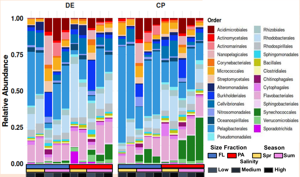
🖼️ Figure description
Today’s figure represents the final, polished visualization generated in R using taxonomic abundance tables derived from Kaiju. The stacked bar plot shows relative abundances at the order level, enabling direct comparison of community composition across samples.
All data processing and visualization were performed using R (v4.x) with packages from the tidyverse ecosystem, and both the input data and complete R code are openly available in the project’s GitHub repository for full reproducibility.
📂 Data and code availability: All Kaiju summary tables and R scripts used to generate this figure are available in the GitHub project repository. https://github.com/jojyjohn28/Size_Fractionated_Microbiome_Analysis
📦 R packages used
# Core tidyverse packages
library(ggplot2)   # visualization
library(readxl)    # reading Excel files
library(dplyr)     # data manipulation
library(tidyr)     # data reshaping
📅 Day 3: MetaPhlAn — marker gene-based profiling We will compare MetaPhlAn-derived abundance tables against Kaiju outputs and begin systematic benchmarking across size fractions.