Size Fractionated Microbiome Anlaysis — Day 1: From Raw Reads to Clean Data

🌊 Size Fractionated Microbiome Anlaysis — Day 1

Today, I’m sharing the beginning of a new analysis series focused on a project exploring:

**How resource partitioning and co-occurrence shape functional redundancy in size-fractionated microbiomes from the Delaware and Chesapeake Bays**

Here, I distinguish between free-living and particle-attached microbial fractions, which represent contrasting ecological lifestyles in estuarine environments. This separation allows us to directly test how niche partitioning influences community composition and functional redundancy. All analyses in this project are performed at the shotgun metagenome read level, allowing us to directly examine both total and active microbial communities without marker-gene or PCR biases.

This project has many dimensions to explore. I decided to start with the foundation: total community profiling, before moving on to activity-based (RNA-informed) analyses.

🌊 Total Community Analysis from Metagenomes

From Raw Reads to Clean, Analysis-Ready Data

To do this systematically, I plan to test three different taxonomic profiling tools and ultimately select one robust method to apply consistently across all samples, based on performance and biological interpretability.

But before asking who is there in a metagenome, we must first make sure the data we start with is *clean, reliable, and biologically meaningful.

🔬 What This Series Is About

Shotgun metagenomics allows us to profile entire microbial communities without PCR amplification, capturing:

● Bacteria

● Archaea

This series will walk through multiple approaches for total community profiling from shotgun metagenomes, starting from raw reads and ending with comparative evaluation of methods.

Planned roadmap:

Day 1: Raw read quality control & preprocessing

Day 2: Kaiju — protein-level taxonomic classification

Day 3: MetaPhlAn — marker-gene based profiling

Day 4: mOTUs — genome-resolved profiling + tool comparison + GitHub release

Today, we start at the very beginning.

📅 Day 1 Focus: Raw Metagenome Preprocessing

Transform raw FASTQ files into clean, trimmed reads suitable for downstream community profiling.

Today’s workflow includes:

● Initial inspection of raw metagenomic reads

● Read quality assessment

● Adapter and quality trimming using Trimmomatic

● Generating analysis-ready FASTQ files

1. 📂 Input Data

Typical input for shotgun metagenomics:

This step is often overlooked, but it controls the quality of everything downstream.

sample_R1.fastq.gz
sample_R2.fastq.gz

These are paired-end Illumina reads (e.g., NovaSeq, HiSeq, NextSeq).

2. 🛠️ Tool Installation

FastQC

FastQC is used for visual inspection of read quality.

conda install -c bioconda fastqc

Trimmomatic

Trimmomatic performs adapter removal and quality trimming.

conda install -c bioconda trimmomatic

Make sure you also have the adapter file (e.g. TruSeq3-PE.fa), which is usually included in the Trimmomatic installation.

3. 🔍 Step 1: Initial Quality Check

Before trimming, always inspect raw read quality.

fastqc sample_R1.fastq.gz sample_R2.fastq.gz

Key things to examine:

● Per-base sequence quality

● Adapter contamination

● Overrepresented sequences

● Read length distribution

At this stage, don’t panic — raw reads often look messy, and that’s completely normal.

4. ✂️ Step 2: Trimming & Filtering with Trimmomatic

For metagenomic data, trimming is essential to:

Remove adapters

Trim low-quality bases

Discard very short reads

Example Trimmomatic Command (Paired-End)

trimmomatic PE -threads 16 \
  sample_R1.fastq.gz sample_R2.fastq.gz \
  sample_R1.trimmed.fastq.gz sample_R1.unpaired.fastq.gz \
  sample_R2.trimmed.fastq.gz sample_R2.unpaired.fastq.gz \
  ILLUMINACLIP:TruSeq3-PE.fa:2:30:10 \
  LEADING:3 \
  TRAILING:3 \
  SLIDINGWINDOW:4:15 \
  MINLEN:50

What each parameter does:

● ILLUMINACLIP → removes adapter contamination

● LEADING / TRAILING → trims low-quality bases at read ends

● SLIDINGWINDOW → trims when average quality drops

● MINLEN → removes very short reads

For downstream taxonomic profiling, the paired trimmed reads are typically used.

5. 📊 Step 3: Post-Trimming Quality Check

Always re-run FastQC after trimming:

fastqc sample_R1.trimmed.fastq.gz sample_R2.trimmed.fastq.gz

You should now observe:

● Improved base quality profiles

● Reduced adapter signals

● Cleaner, more consistent reads

📁 Output of Day 1

By the end of Day 1, you should have:

sample_R1.trimmed.fastq.gz
sample_R2.trimmed.fastq.gz

These files are analysis-ready and will be used for all taxonomic profiling approaches in the coming days.

🧠 Why This Step Matters

Every profiling tool (Kaiju, MetaPhlAn, mOTUs) assumes:

● High-quality reads

● Minimal sequencing errors

● No adapter contamination

Skipping or rushing preprocessing can:

● Inflate false positives

● Bias abundance estimates

R● educe mapping accuracy

👉 Clean input = trustworthy biological conclusions

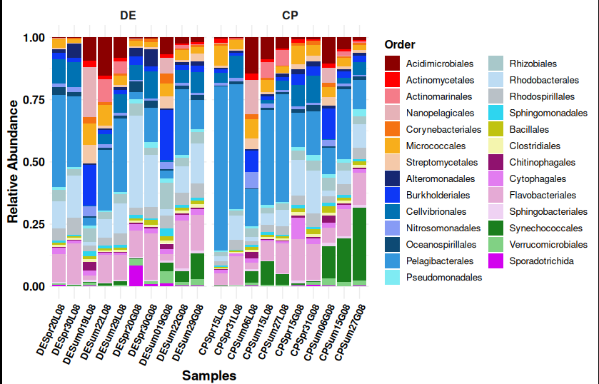
On day 2 we will use Kaiju for exploring total community analysis.

> The figure attached here is generated from Kaiju outputs.
> More details about this analysis will be covered in Day 2.