From Genome Assembly to Novel Species: A Step-by-Step Genomic Workflow
🧬 From Genome Assembly to Novel Species: A Step-by-Step Genomic Workflow
Case study: Winogradskyella sp. PC_D3_3
Today’s post steps slightly away from community profiling and focuses on a question every microbial genomicist eventually faces:
How do we confidently determine whether a newly sequenced genome represents a novel bacterial species?
Using a newly assembled long-read genome (Winogradskyella sp. PC_D3_3), I walk through a complete, reproducible workflow—from assembly quality checks to taxonomic placement, genomic similarity metrics (ANI, AAI, dDDH), and functional interpretation.
This is the same logic used for NCBI submissions, Genome Resource Announcements, and formal species descriptions.
Step 1: 🔍 Long-Read Sequence Quality Assessment with NanoPlot
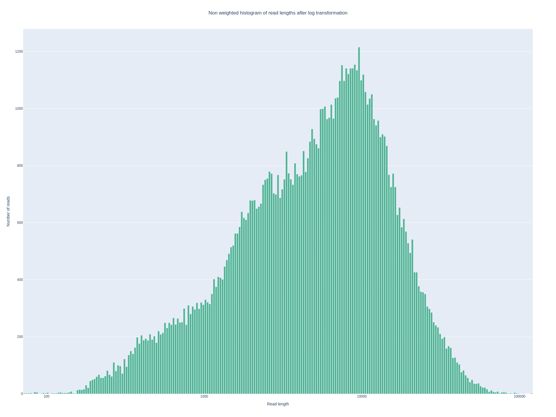
Before genome assembly, assessing the quality of long-read sequencing data is critical to ensure sufficient read length, coverage, and overall data reliability. For Oxford Nanopore Technologies (ONT) reads, I used NanoPlot to visualize read length distributions, quality scores, and cumulative yield.
Why NanoPlot?
● NanoPlot provides a rapid overview of key long-read metrics, including:
● Read length distribution (mean, N50, max length)
● Per-read quality score distribution
● Cumulative sequencing yield
● Read length vs. quality relationships
These metrics help determine whether the dataset is suitable for de novo assembly and whether additional filtering or re-sequencing is required. 🔧 Installation (Linux / Conda)
conda install -c bioconda nanoplot
▶️ Running NanoPlot
NanoPlot \
  --fastq PC_D3_3.fastq.gz \
  --outdir nanoplot_PC_D3_3 \
  --threads 8
📊 Interpreting the Output
Key outputs generated by NanoPlot include:
● Read length histogram — confirms the presence of long reads necessary for resolving repeats
● Read quality distribution — ensures sufficient base-calling accuracy
● Cumulative yield plot — verifies total sequencing depth
● Length vs. quality scatter plots — identifies potential low-quality long reads
🧪 Step 2: Long-Read Genome Assembly
The genome was assembled using Oxford Nanopore long reads and Flye, which is well suited for circular bacterial chromosomes.
python flye \
  --nano-raw PC_D3_3.fastq.gz \
  --threads 32 \
  --out-dir lr
Assembly summary:
● Genome size: 4.21 Mb
● Contigs: 1
● Coverage: ~170×
● Topology: Circular
Flye produced a single, high-coverage contig, consistent with a complete bacterial chromosome.
📊 Step 3: Assembly Quality Assessment
QUAST
quast.py PC_D3_3.fasta -o quast_output
Key statistics:
● Contigs: 1
● N50: 4,212,977 bp
● GC content: 33.32%
● Ns: 0
CheckM
checkm lineage_wf -x fa lr checkm_out
● Completeness: 99.28%
● Contamination: 1.09%
● Strain heterogeneity: 0%
✔ High completeness and low contamination support downstream taxonomic claims.
🧬 Step 4: Genome Annotation Overview
Prokka
prokka PC_D3_3.fasta --outdir prokka
Prokka gives overall annotations.
● CDS: 3,748
● rRNA: 12
● tRNA: 48
● tmRNA: 1
DRAM (functional overview)
DRAM.py annotate -i PC_D3_3.fasta -o dram
DRAM.py distill -i dram/annotations.tsv -o dram/genome_summaries
Why DRAM? It provides:
● CAZyme profiles
● Central metabolism
● Transporters
● Secondary metabolites
● Polysaccharide utilization potential
This goes far beyond simple gene counts.
🧭 Step 5: Taxonomic Placement with GTDB-Tk
To assign standardized taxonomy and place the genome within the Genome Taxonomy Database (GTDB) framework, I used GTDB-Tk, which classifies genomes based on a curated set of conserved marker genes and reference phylogenies.
1️⃣ Identify marker genes
gtdbtk identify \
  --genome_dir /scratch/jojyj/win_dec11/lr \
  --out_dir /scratch/jojyj/win_dec11/gtdbtk/identify \
  --extension fasta \
  --cpus 32
What this does: This step scans the genome for GTDB’s conserved bacterial marker genes and prepares them for downstream phylogenetic placement.
2️⃣ Align marker genes
gtdbtk align \
  --identify_dir /scratch/jojyj/win_dec11/gtdbtk/identify \
  --out_dir /scratch/jojyj/win_dec11/gtdbtk/align \
  --cpus 32
Identified marker genes are aligned against GTDB reference alignments, enabling consistent phylogenetic comparison across genomes.
3️⃣ Classify the genome
gtdbtk classify \
  --genome_dir /scratch/jojyj/win_dec11/lr \
  --align_dir /scratch/jojyj/win_dec11/gtdbtk/align \
  --out_dir /scratch/jojyj/win_dec11/gtdbtk/classify \
  -x fasta \
  --cpus 32 \
  --mash_db /scratch/jojyj/win_dec11/gtdbtk
This step assigns taxonomy to the genome by placing it into the GTDB reference tree using both phylogenetic placement and Mash-based genome distance estimates.
📄 Key Output: GTDB-Tk Classification Table
The classification table produced here is critical for the next steps. File of interest:
gtdbtk.bac120.summary.tsv
(or classify.csv, depending on GTDB-Tk version)
This table contains:
● GTDB taxonomy (domain → species)
● Closest GTDB reference genomes
● ANI-based placement confidence
● Novelty flags (e.g., no species assignment)
How this table is used next (important)
The GTDB-Tk classification output is typically used to:
● Identify closest reference genomes
● Extract GTDB/NCBI accession IDs
● Download ~10–20 closely related genomes using the NCBI CLI
● Perform ANI, AAI, and dDDH comparisons
📥 Step 6: Download Closely Related Genomes (NCBI CLI)
To test novelty, we compare PC_D3_3 against closely related reference genomes. Install NCBI datasets (Linux)
conda install -c conda-forge ncbi-datasets-cli
Download reference genomes
datasets download genome taxon "Winogradskyella" \
  --assembly-level complete \
  --filename winogradskyella_refs.zip
Here I used the classify table created using GTDBtk classify. Unzip and retain ~10–20 representative genomes.
🧮 Step 7: ANI Analysis (FastANI)
Average Nucleotide Identity (ANI) comparisons between Winogradskyella sp. PC_D3_3 and representative reference genomes:
Install FastANI
conda install -c bioconda fastani
Run ANI
fastANI \
  -q PC_D3_3.fasta \
  -r reference_genomes/*.fna \
  -o ani_results.txt
my output | Reference genome | ANI (%) | | ———————- | ——- | | W. psychrotolerans B | 85.82 | | W. thalassocola | 85.38 | | W. pacifica | 84.96 | | W. marina | 81.85 |
Observed ANI range: 81.2% – 85.8% All ANI values fall well below the 95–96% species threshold, supporting designation as a novel species.
📌 Interpretation
● Species cutoff: 95–96% ANI
● All values fall far below this threshold
● ➡ PC_D3_3 is not any known Winogradskyella species
🧬 Step 8: AAI Analysis (CompareM)
Average Amino Acid Identity is also used compare between the closely related genomes.
Install CompareM
conda install -c bioconda comparem
Run AAI
comparem aai_wf PC_D3_3.faa refs/ aai_out
| Reference genome | Mean AAI (%) |
|---|---|
| W. thalassocola | 87.11 |
| W. pacifica | 86.86 |
| W. psychrotolerans | 86.49 |
| W. undariae | 82.37 |
AAI values are above genus-level cutoffs but below species-level thresholds, confirming genus-level placement with species-level novelty.
Observed AAI range: 81.7% – 87.1%
📌 Interpretation
Species cutoff: ~95%
Genus cutoff: ~65–75%
➡ Confirms same genus, novel species
🧬 Step 9: Digital DNA–DNA Hybridization (GGDC)
dDDH was calculated using the DSMZ GGDC web platform (Formula 2). Digital DNA–DNA hybridization (dDDH) estimates: | Reference genome | dDDH (%) | | ———————- | ——– | | W. psychrotolerans B | 29.0 | | W. thalassocola | 28.8 | | W. pacifica | 27.8 | | W. costae | 25.9 |
All values are far below the 70% dDDH species cutoff, with near-zero probabilities of species identity.
Observed dDDH values: 23–29%
📌 Species cutoff: 70% 📌 Probability of species identity: 0–7%
➡ Definitive evidence for novel species status
Takeaway
Consistent evidence from ANI, AAI, and dDDH analyses confirms that Winogradskyella sp. PC_D3_3 represents a novel species, motivating careful cross-device synchronization of genome data, scripts, and analyses.
🧠 Functional Interpretation (DRAM Highlights)
Winogradskyella sp. PC_D3_3 is:
● A polysaccharide-degrading marine heterotroph
● Rich in CAZymes (alginate lyases, amylases, pectinases)
● Equipped with diverse ABC and Mce transporters
● Motile (MotB), suggesting particle association
● Carries CRISPR–Cas9, indicating viral pressure
● Strongly adapted to macroalgal and particulate organic matter
This functional profile aligns with a particle-attached, algal-detritus–associated lifestyle in coastal systems.
🧠 Take-Home Messages
● Never rely on taxonomy alone—use ANI, AAI, and dDDH together
● Long-read assemblies dramatically simplify genome interpretation
● DRAM adds ecological meaning beyond taxonomy
● Genomic novelty is strongest when multiple metrics converge
todays figure shows non weighted histogram of read length of current novel genome (after log transformation) from nanoplot