Amplicon Week — Day 3: Visualization & Ecological Analysis Using QIIME2 + Microeco (R)
🌱 Amplicon Week — Day 3
Visualization & Ecological Analysis Using QIIME2 + Microeco (R)
After completing the QIIME2 core analysis (Day 2), today we move into the visualization and ecological interpretation phase using Microeco, one of the most flexible and modern R packages for microbial community data mining.
This workflow works for 16S, ITS, 18S, 12S, and COI — as long as you export your ASV table, taxonomy, tree, and metadata from QIIME2.
📦 What is Microeco?
Microeco is an R package designed for modular, flexible, comprehensive microbial ecological analysis using an R6 object-based framework.
⭐ Key features:
Creation of a unified microtable object
● Data cleaning & normalization
● Taxonomic visualization (barplots, heatmaps, composition)
● Venn diagrams
● Alpha & Beta diversity
● Differential abundance testing
● Co-occurrence network analysis
● Environmental data integration
● Supports multiple platforms: QIIME2, QIIME, HUMAnN, Kraken2, Phyloseq, MetaPhlAn, etc.
Microeco essentially brings the entire downstream microbial ecology workflow into one consistent R environment.
🧩 1. Creating a Microeco microtable object from QIIME2 outputs
Microeco expects the following input files:
| File | Source | Format |
|---|---|---|
| ASV table | QIIME2 table.tsv | ASV × samples |
| Taxonomy table | taxonomy.tsv | ASV taxonomy |
| Representative sequences | (optional) | FASTA |
| Phylogenetic tree | rooted-tree.nwk | Newick |
| Sample metadata | user-provided | TSV |
After exporting in Day 2, you will have:
feature-table.tsv
taxonomy.tsv
tree.nwk
metadata.tsv
A. Option 1 — Using file2meco (recommended)
Microeco provides a companion package file2meco to directly read QIIME2 files into microtable.
install.packages("microeco")
devtools::install_github("ChiLiubio/file2meco")

library(file2meco)

mt <- file2meco::qiime2_to_meco(
  feature_table = "feature-table.tsv",
  taxonomy = "taxonomy.tsv",
  tree = "tree.nwk",
  metadata = "metadata.tsv"
)
This automatically:
● Cleans taxonomy
● Aligns sample names
● Creates the microtable object
B. Option 2 — Manual creation (phyloseq-style)
If you want full control:
library(microeco)
library(tidyverse)

otu <- read.table("feature-table.tsv", header = TRUE, row.names = 1, sep = "\t")
tax <- read.table("taxonomy.tsv", header = TRUE, row.names = 1, sep = "\t")
meta <- read.table("metadata.tsv", header = TRUE, row.names = 1, sep = "\t")
tree <- ape::read.tree("tree.nwk")

# Clean taxonomy (important!)
tax <- tidy_taxonomy(tax)

mt <- microtable$new(
  otu_table = otu,
  tax_table = tax,
  sample_table = meta,
  phylo_tree = tree
)

mt
🌈 2. Taxonomic Composition Analysis (Barplots)
Visualizing relative abundance across samples or groups. Create object:
t1 <- trans_abund$new(dataset = mt, taxrank = "Phylum", ntaxa = 20)
Plot:
t1$plot_bar(
  others_color = "grey70",
  facet = "Group",
  xtext_keep = FALSE,
  legend_text_italic = FALSE
)
✔ Shows top abundant phyla ✔ Automatically groups the rest as “Others” ✔ Facets by metadata (e.g., treatment, season, habitat) ✔ Can create same for top families, genus or species.
🟣 3. Venn Diagram (Shared ASVs/OTUs)
Useful for comparing core taxa across groups.
v1 <- trans_venn$new(dataset = mt, group = "Group")
v1$plot_venn()
📏 4 Diversity analysis
4.1 Microeco makes this very simple:
Microeco makes this very simple:
adiv <- trans_alpha$new(dataset = mt, group = "Group")
adiv$plot_alpha(boxplot = TRUE)
or individual metrics:
adiv$plot_metric("Shannon")
adiv$plot_metric("Chao1")
can be modified to include the ststistical analysis.
4.2 Beta Diversity (PCoA / NMDS)
Bray–Curtis PCoA:
bdiv <- trans_beta$new(dataset = mt, group = "Group", distmethod = "bray")
bdiv$plot_ordination(method = "PCoA")
NMDS example:
bdiv$plot_ordination(method = "NMDS")
Clustering patterns often reveal:
● treatment effects
● environmental gradients
● size fraction differences
● seasonal signatures
For incorporating ststistical analysis for diversity; please refer diversity_statistics.R in day3 of github project.
✅ WHAT THIS SCRIPT PRODUCES
Alpha diversity
● alpha_KruskalWallis_results.csv
● alpha_Wilcoxon_results.csv
● alpha_ANOVA_results.csv
Beta diversity
● beta_PERMANOVA_BrayCurtis.csv
● beta_Betadisper_BrayCurtis.csv
● Complete results object
● diversity_statistics.RData
📊 5. Differential Abundance
Microeco can run LEfSe-style analysis internally.
lf <- trans_diff$new(dataset = mt, group = "Group", method = "lefse")
lf$plot_diff_bar()
This identifies biomarkers at different taxonomic levels.
🔭 Microeco Can Do Even More
In this post, I focused on the core ecological analyses: composition, diversity, differential abundance, and basic networks. But Microeco can do much more, including:
● RDA / CCA and other ordination methods integrating environmental variables
● Correlation-based analyses (taxa–taxa, taxa–environment)
● WGCNA-style module detection and co-occurrence structure
● Functional prediction workflows and downstream visualization
For a deeper dive into these advanced features, I highly recommend the official tutorial: 👉 https://chiliubio.github.io/microeco_tutorial/
Keep in mind that many of these analyses are also possible directly in QIIME2. For more details on QIIME2-based visualizations and diversity analyses, see:
👉 qiime2_visualization.md in the Day 3 folder of the GitHub project https://github.com/jojyjohn28/AmpliconWeek_2025
If you are interested in trying Microeco, I’ve included all the required base files in my repository, along with a fully running R script. You can find: feature-table.tsv taxonomy.tsv tree.nwk metadata.txt and Dec10_microeco.R
These files allow you to reproduce the entire workflow exactly as shown.
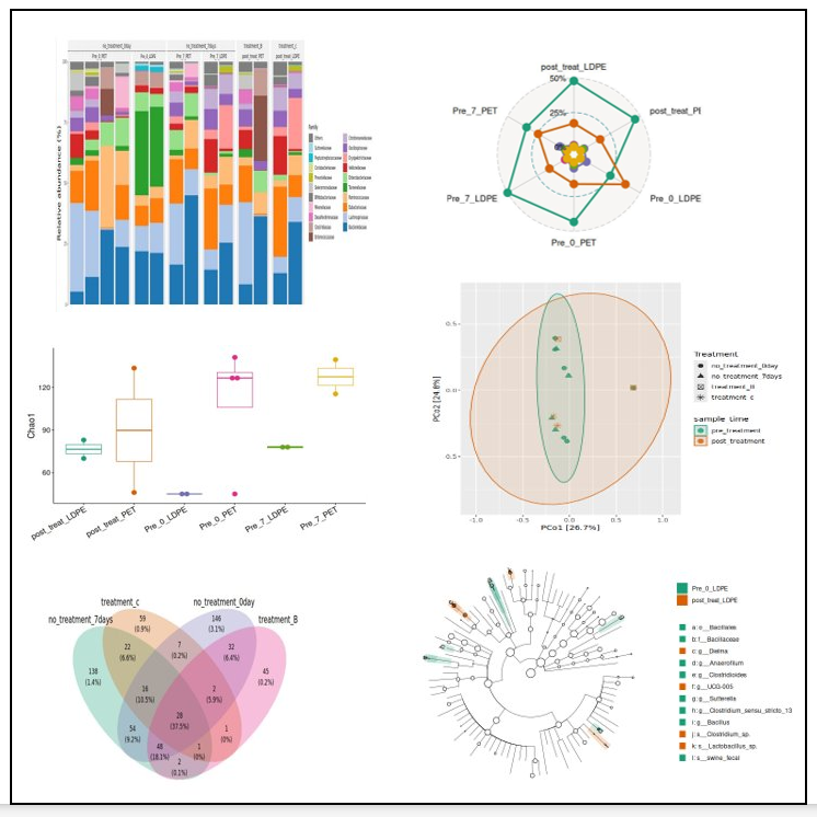
Today’s image features visualizations I created myself using Microeco.
Thank you to the Campbell Lab’s graduate student seminar series — especially Dinu and Nichole — for the presentation on Microeco