Day 6: Specialized Genomic Functions

Estimated Time: 8-12 hours

Difficulty: Advanced

Prerequisites: Day 5 (Annotation)

📚 Table of Contents

Introduction
Secondary Metabolites
Antimicrobial Resistance
Carbohydrate-Active Enzymes
Prophages & Viruses
CRISPR Systems
Mobile Genetic Elements
Protein Domains
Comparative Analysis
Best Practices

🎯 Introduction

Welcome to Day 6! After basic annotation (Day 5), it’s time to discover hidden genomic treasures - specialized functions that make organisms unique.

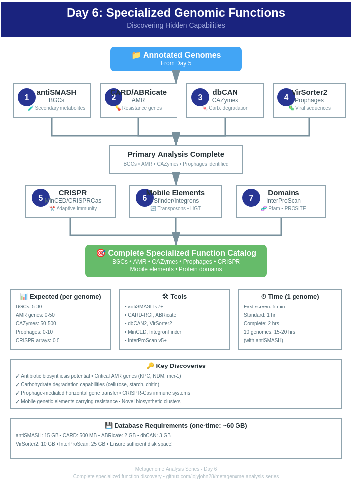
Today’s discoveries:

🧪 Secondary metabolites - Antibiotics, toxins, signaling molecules
💊 Antimicrobial resistance - AMR genes and mechanisms
🍬 CAZymes - Carbohydrate degradation capabilities
🦠 Prophages - Integrated viral sequences
✂️ CRISPR systems - Bacterial immune systems
🔄 Mobile elements - Transposons, insertion sequences
🧬 Protein domains - Functional motifs and structures

Why This Matters

Basic annotation tells you:

This is a kinase
This is a transporter

Specialized analysis reveals:

This organism produces penicillin
This strain is resistant to carbapenems
This microbe can degrade cellulose
This genome contains CRISPR-Cas9

🧪 Secondary Metabolites

antiSMASH: Biosynthetic Gene Cluster Detection

antiSMASH (antibiotics & Secondary Metabolite Analysis SHell) is the gold standard for BGC detection.

Installation

# Create environment
conda create -n antismash -c bioconda antismash
conda activate antismash

# Download databases (~15 GB)
download-antismash-databases

Basic Usage

conda activate antismash

# Single genome
antismash \
    --output-dir antismash_output/genome1 \
    --genefinding-tool prodigal \
    --cpus 8 \
    genome1.gbk

# With all features enabled
antismash \
    --output-dir antismash_output/genome1 \
    --genefinding-tool prodigal \
    --knownclusterblast \
    --subclusterblast \
    --clusterblast \
    --smcog-trees \
    --cpus 8 \
    genome1.gbk

Input formats:

GenBank (.gbk) - recommended
FASTA (.fa) - requires gene finding

antiSMASH Output

antismash_output/genome1/
├── genome1.gbk                    # Annotated genome
├── genome1.json                   # Machine-readable results
├── index.html                     # Interactive visualization
├── regions.js                     # BGC regions
├── knownclusterblast/            # Hits to known BGCs
└── svg/                          # Cluster visualizations

BGC types detected:

Polyketides (PKS)
Non-ribosomal peptides (NRPS)
Terpenes
Bacteriocins
Siderophores
RiPPs (Ribosomally synthesized and Post-translationally modified Peptides)

Parse antiSMASH Results

please use parse_antismash.py from Day 6 →

BiG-SCAPE: BGC Similarity Analysis

BiG-SCAPE compares BGCs across multiple genomes to identify families.

Installation

conda create -n bigscape -c bioconda bigscape
conda activate bigscape

Usage

# Collect all BGC GenBank files from antiSMASH
mkdir bigscape_input
cp antismash_output/*/regions/*.gbk bigscape_input/

# Run BiG-SCAPE
bigscape \
    -i bigscape_input \
    -o bigscape_output \
    --pfam_dir ~/pfam_database \
    --cores 8 \
    --mode auto

# Visualize
firefox bigscape_output/network_files/index.html

BiG-SCAPE output:

BGC families (grouped by similarity)
Network visualization
Comparative analysis across genomes

💊 Antimicrobial Resistance

CARD-RGI: Comprehensive AMR Database

RGI (Resistance Gene Identifier) uses CARD database for AMR detection.

Installation

conda create -n rgi -c bioconda rgi
conda activate rgi

# Download CARD database
rgi load --card_json ~/card_database/card.json

# Verify
rgi database --version

Usage

conda activate rgi

# Predict AMR from proteins
rgi main \
    --input_sequence proteins.faa \
    --input_type protein \
    --output_file rgi_output \
    --clean \
    --num_threads 8

# From nucleotides (slower but more sensitive)
rgi main \
    --input_sequence genome.fa \
    --input_type contig \
    --output_file rgi_output \
    --clean \
    --num_threads 8 \
    --include_loose

RGI output columns:

ORF_ID
ARO (Antibiotic Resistance Ontology)
Drug Class
Resistance Mechanism
AMR Gene Family

Parse RGI Results

Use parse_rgi.py from Day 6 →

ABRicate: Fast AMR Screening

ABRicate screens multiple AMR databases quickly.

Installation

conda create -n abricate -c bioconda abricate
conda activate abricate

# Update databases
abricate-get_db --db all

Usage

conda activate abricate

# Screen against all databases
abricate genome.fa > abricate_results.tab

# Specific database
abricate --db card genome.fa > card_results.tab
abricate --db resfinder genome.fa > resfinder_results.tab
abricate --db vfdb genome.fa > virulence_results.tab

# Batch processing
abricate genomes/*.fa > all_genomes_amr.tab

# Summary
abricate --summary all_genomes_amr.tab > amr_summary.tab

Available databases:

card (CARD)
resfinder (ResFinder)
ncbi (NCBI AMRFinderPlus)
argannot
megares
vfdb (Virulence factors)
plasmidfinder

🍬 Carbohydrate-Active Enzymes (CAZymes)

dbCAN2: CAZyme Annotation

dbCAN identifies enzymes that degrade, modify, or create carbohydrates.

Installation

conda create -n dbcan -c bioconda dbcan
conda activate dbcan

# Download databases
dbcan_build --help

Usage

conda activate dbcan

# Run dbCAN
run_dbcan \
    proteins.faa \
    protein \
    --out_dir dbcan_output \
    --db_dir ~/dbcan_db \
    --tools all \
    --threads 8

# Output: dbcan_output/overview.txt

CAZyme families:

GH - Glycoside Hydrolases (breakdown)
GT - Glycosyl Transferases (synthesis)
PL - Polysaccharide Lyases
CE - Carbohydrate Esterases
AA - Auxiliary Activities
CBM - Carbohydrate-Binding Modules

Parse dbCAN Results

Use parse_dbcan.py from Day 6 →

🦠 Prophages & Viruses

VirSorter2: Viral Sequence Detection

VirSorter2 identifies viral sequences in genomes and metagenomes.

Installation

conda create -n virsorter2 -c bioconda virsorter=2
conda activate virsorter2

# Setup database
virsorter setup -d ~/virsorter2-db -j 4

Usage

conda activate virsorter2

# Run VirSorter2
virsorter run \
    -i genome.fa \
    -w virsorter2_output \
    --min-length 5000 \
    --min-score 0.5 \
    -j 8 \
    all

# High-confidence viral sequences
cat virsorter2_output/final-viral-boundary.tsv

VirSorter2 output:

Prophage regions
Viral score (0-1)
Boundary coordinates
Gene content

PHASTER: PHAge Search Tool Enhanced Release

PHASTER identifies prophages with detailed annotation.

Note: PHASTER is primarily a web service.

Web interface: https://phaster.ca/

Alternative: Use VirSorter2 + CheckV

# CheckV for viral genome quality
conda create -n checkv -c bioconda checkv
conda activate checkv

# Download database
checkv download_database ~/checkv-db

# Run CheckV on VirSorter2 results
checkv end_to_end \
    virsorter2_output/final-viral-combined.fa \
    checkv_output \
    -d ~/checkv-db \
    -t 8

✂️ CRISPR Systems

CRISPRCasFinder: Detect CRISPR-Cas Systems

# Installation
conda create -n crisprcasfinder -c bioconda crisprcasfinder
conda activate crisprcasfinder

# Run
CRISPRCasFinder.pl \
    -in genome.fa \
    -out crispr_output \
    -cas \
    -keep

MinCED: Simple CRISPR Detection

conda create -n minced -c bioconda minced
conda activate minced

# Quick CRISPR detection
minced genome.fa crispr_output.txt

# Parse results
grep "CRISPR" crispr_output.txt

CRISPR system types:

Type I (most common in bacteria)
Type II (Cas9 - CRISPR editing)
Type III
Type IV-VI (rare)

🔄 Mobile Genetic Elements

ISfinder: Insertion Sequences

# Use ABRicate with custom IS database
abricate --db isfinder genome.fa > is_results.tab

# Or BLAST against ISfinder database
blastn \
    -query genome.fa \
    -db ~/isfinder_db/ISfinder \
    -outfmt 6 \
    -num_threads 8 \
    > is_blast.out

Integron Finder

conda create -n integron_finder -c bioconda integron_finder
conda activate integron_finder

# Find integrons
integron_finder \
    --local-max \
    --cpu 8 \
    genome.fa

Integrons contain:

Integration sites
Gene cassettes
Often AMR genes

🧬 Protein Domains & Functions

InterProScan: Comprehensive Domain Analysis

InterProScan searches multiple protein signature databases.

Installation

# Large download - recommend using web service
# Or install locally:
wget ftp://ftp.ebi.ac.uk/pub/software/unix/iprscan/5/5.XX-XX.X/interproscan-5.XX-XX.X-64-bit.tar.gz
tar -xzf interproscan-5.XX-XX.X-64-bit.tar.gz

Usage

# Run InterProScan
interproscan.sh \
    -i proteins.faa \
    -f TSV,GFF3 \
    -o interproscan_output \
    --cpu 8 \
    --goterms \
    --pathways

Databases searched:

Pfam (protein families)
PROSITE (patterns)
PRINTS
SMART
TIGRFAMs
PANTHER
Gene3D
Superfamily

Parse InterProScan

Use parse_ipr.py from Day 6 →

📊 Comprehensive Analysis Workflow

Complete Specialized Function Pipeline

Use comprehensive_analysis.sh from Day 6 →

📈 Comparative Analysis

Compare Specialized Functions Across Genomes

Use compare_specialized_functions.py from Day 6 →

💡 Best Practices

Before Analysis

✅ Have complete gene predictions (Prodigal/Prokka)
✅ Use GenBank format for antiSMASH
✅ Check genome quality (comp >80%, cont <5%)
✅ Ensure databases are updated

During Analysis

✅ Run tools in priority order (fast → slow)
✅ Use multiple tools for AMR (RGI + ABRicate)
✅ Save intermediate files
✅ Document tool versions

After Analysis

✅ Validate hits manually (especially AMR)
✅ Check for false positives
✅ Cross-reference with literature
✅ Visualize results

🔧 Troubleshooting

antiSMASH: No BGCs detected

# Check input format
head genome.gbk

# Try with relaxed detection
antismash --minimal ...

# Ensure genome is annotated

RGI: No results

# Update CARD database
rgi load --card_json ~/card_database/card.json

# Try --include_loose for more hits
rgi main --include_loose ...

dbCAN: Low CAZyme count

# Use all three tools
run_dbcan --tools all ...

# Check protein quality
grep ">" proteins.faa | wc -l

📈 Expected Results

Typical Findings per Genome

Feature	Typical Range
BGCs	5-30
AMR genes	0-50
CAZymes	50-500
Prophages	0-10
CRISPR arrays	0-5
Integrons	0-5

Visulaizations

📊 1. bgc_heatmap.R - BGC Distribution

What it does:

● Visualizes antiSMASH BGC distributions across genomes ● Creates 3 heatmap variants (basic, custom colors, annotated) ● Includes toy data built-in ● Automatic clustering by BGC similarity

Outputs:

● bgc_heatmap_basic.pdf - Simple clustered heatmap ● bgc_heatmap_custom.pdf - Custom gradient (white → gold → red → purple) ● bgc_heatmap_annotated.pdf - With annotations for BGC richness ● bgc_summary.csv - Summary statistics

Toy data included: 15 genomes × 9 BGC types

🍬 2. cazyme_bubble_plot.R - CAZyme Analysis

What it does:

● Creates bubble plots showing CAZyme family distributions ● Bubble size = CAZyme count ● Color = Genome completion percentage ● Includes heatmap and bar plot variants ● Analyzes degradation capabilities

Outputs:

● cazyme_bubble_plot.pdf - Main bubble visualization ● cazyme_bubble_plot_alt.pdf - Alternative color scheme ● cazyme_total_barplot.pdf - Total counts by taxonomic order ● cazyme_heatmap.pdf - Clustered heatmap ● cazyme_summary.csv - Summary with degradation analysis

Toy data included: 12 taxonomic orders × 6 CAZyme families

All R-codes available in *Day 6 →

Processing Time (8-core laptop)

Tool	Single Genome	10 Genomes
antiSMASH	30-60 min	8-10 hrs
RGI	5-10 min	1-2 hrs
ABRicate	1-2 min	15-20 min
dbCAN	10-20 min	2-3 hrs
VirSorter2	20-40 min	5-7 hrs
InterProScan	1-2 hrs	15-20 hrs

✅ Success Checklist

📚 Key Resources

Tools & Databases

➡️ What’s Next?

Congratulations! You’ve discovered the specialized capabilities of your genomes!

Next steps:

Comparative genomics
Pangenome analysis
Phylogenomics
Publication!

Repo for today’s code and other details

🔗 Day 6 →

Last updated: February 2026

day6 mg